OpenMMS Software

OpenMMS Open-Source Software License

This documentation describes Open-Source Software and is licensed under the GNU GPL-3 license.
View the OpenMMS Open-Source Licenses for more details.

In addition to the OpenMMS hardware, a software suite of open-source applications is also at the core of the OpenMMS Project. Visit the OpenMMS GitHub page for details on how to install and configure the OpenMMS open-source software applications and all the supporting software applications.

---

OpenMMS Operating System (OMOS)

To simplify the steps needed to get a Raspberry Pi 4 Model B computer installed with all the necessary OpenMMS software and dependencies, a complete Operating System image file has been created. The OMOS image is based on the Raspberry Pi OS (previously called Raspbian) version Feb. 2020, with system upgrades applied in June 2020. The image file can be directly written to a microSD card and then installed in the Raspberry Pi computer.

As mobile mapping datasets can be very large, it is recommended to use a minimum 32GB microSD card with speed class 10 or U3. For readers new to the concept of how to write an OS image file to an SD card, the Raspberry Pi Foundation provides a simple computer application, for free, that performs this task. Click here to download the Raspberry Pi Imager application.

Click here to download the latest OpenMMS OS (for sensors with a VLP-16 lidar)
Click here to download the latest OpenMMS OS (for sensors with a Livox lidar)

Important

• The extracted OpenMMS OS image file is ~4GB in size.
  

• The root filesystem is automatically expanded to occupy the remaining space on the microSD card after the 1st system boot-up.
  

• All subsequent system boot-ups (i.e., starting with the 2nd boot-up) will realize the increased filesystem size.
  

• The RPi Device Name is OpenMMS, and its static IP address is 192.168.1.81
  

• If an interested user wants to SSH into the RPi, use username : password = openmms : $mmnep0 (ends with the number zero).
  

• DO NOT CHANGE THE USERNAME OR PASSWORD, OR THE REAL-TIME CODE WILL BREAK!

---

OpenMMS Applications

Attention

Please follow the OpenMMS Software installation and configuration instructions found HERE , in order to ensure the OpenMMS data processing and quality assurance strategies can be successfully implemented on a user’s computer.

Most of the applications are written in Python3, and tested within Windows 10 and Mac OS 10.14 environments. Though the applications have not been directly tested within the Debian or Ubuntu Linux distros (yet), they should work. Note: A current development effort (as of May 2020) is underway to leverage NVidia CUDA GPU processing techniques within the OpenMMS software suite for the Windows 10 OS. Future versions of the OpenMMS applications will support NVidia CUDA processing, when possible.

The following software applications all link to the OpenMMS GitHub page, so they will always refer to each application’s most current version. They are included here solely for reference. Click on an application to view the code.

Table S1: OpenMMS Software Applications
Real-Time Applications	Post-Processing Applications	Calibration Applications
Intervalometer Sketch [C++] Sensor Controller (VLP-16) Sensor Controller (Livox)	PCAP Check (VLP-16) PCAP Check (Livox) TRAJ Convert Georeference (VLP-16) Georeference (Livox) Preprocess Images Colorize	Lidar Calibration (VLP-16) Lidar Calibration CUDA (VLP-16) Lidar Calibration (Livox) Lidar Calibration CUDA (Livox) Camera Calibration (a6000)
		Download Only (No code view)
		GNSS Antenna Lever-arms [Excel]

QUICK DESCRIPTION OF EACH APPLICATION

i. Intervalometer Sketch - Receives input from the Sensor Controller application and triggers the mapping camera at the specified time interval.
ii. Sensor Controller - Monitor the state of the sensor’s INPUT pushbutton for user commands and control the hardware accordingly.
iii. PCAP Check - Analyzes the collected VLP-16 lidar dataset and reports quality assurance metrics.
iv. TRAJ Convert - Converts the collected real-time trajectory dataset into the OpenMMS trajectory file format
v. Georeference - Generates the point cloud dataset from the collected lidar and trajectory datasets.
vi. Preprocess Images - Analyzes the collected images and matches them to the correct timing event and can resize/undistort the images.
vii. Colorize - Assigns R,G,B values to each point within the point cloud dataset based on the collected images.
viii. Lidar Calibration - Analyzes planar sections within the point cloud dataset and estimates the lidar sensor’s boresight misalignment angles.
ix. Camera Calibration - Analyzes the images’ positions and orientations, and estimates the camera’s external calibration parameters.
x. GNSS Antenna Lever-arms - an Excel template for entering the calibration procedure observations and computing the lever-arm offsets.

---

Data Processing Workflow

1. Overview

The current suite of OpenMMS open-source software applications are all executed via the command-line interface (CLI). Future development plans include creating a GUI for the suite of applications, but CLI is currently all that is available. However, rather than expecting a user to manually type out (and remember) each command, a set of Batch scripts (for Windows users) and Bash scripts (for Mac/Linux users) have been created. These scripts, from here on referred to as trigger files, contain all the needed processing options (all set to default values) for each of the OpenMMS Python3-based applications. The OpenMMS data processing workflow requires the necessary trigger files to be copied to each directory that contains OpenMMS datasets that need to be processed. Then, the processing options inside each trigger file can be edited as required. Lastly, to execute the processing, the trigger file simply needs to be double-clicked.

This processing approach is nowadays considered to be unconventional, which the author understands. To improve the quality of these instructions, two exhaustive data processing tutorials are included. Tutorial #1 focuses on Velodyne VLP-16 lidar data, while tutorial #2 focuses on Livox MID-40 lidar data. The tutorials work through each of the OpenMMS data processing and calibration steps from start to finish. Each step is documented in detail and includes relevant computer screenshots, videos, helpful tips, and common problems to avoid.

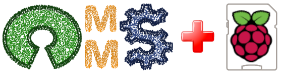
The following flowchart illustrates where each of the OpenMMS open-source software applications is used within the data processing workflow.

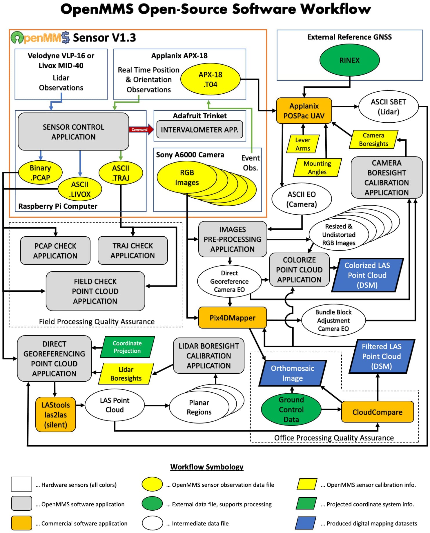
Fig 1-1. OpenMMS open-source software workflow

---

2. Data Processing Tutorial #1

Attention

The demo project’s lidar data was collected using an OpenMMS sensor with a Velodyne VLP-16 lidar scanner. Therefore, the following documentation discusses and showcases the OpenMMS data processing workflow for sensors with a Velodyne VLP-16.

See Data Processing Tutorial #2 (below) if you are interested in the OpenMMS data processing workflow using Livox MID-40 lidar data.

2.1 Demo Project Data (VLP-16)

OpenMMS Open Data License

Copyright Ryan G. Brazeal 2020.

This OpenMMS Demo Project Data (VLP-16) is made available under the Open Database License: https://opendatacommons.org/licenses/odbl/1.0/. Any rights in individual contents of the data are licensed under the Database Contents License: https://opendatacommons.org/licenses/dbcl/1.0/.

Click Here to Download the OpenMMS Demo Project Data (VLP-16), approx. 5 GB .zip archive

The Demo Project Data (VLP-16) is for an RPAS-Lidar mapping project collected with an earlier version of the OpenMMS sensor (you may notice the differences in some of the Applanix mounting angles and lever-arm offsets). The data was collected on June 10th, 2019, over a rural farmyard near Lumsden, Saskatchewan, Canada. The OpenMMS sensor was flown on a DJI M600 Pro RPAS at an altitude of ~ 40 m above ground level (AGL), at a horizontal speed of ~ 5 m/s, mapping images were taken every ~ 2 sec, and a video of the flight was recorded. The included OpenMMS datasets are:

1. GNSS-INS observations from an Applanix APX-18 sensor, .T04 file

2. Lidar observations from a Velodyne VLP-16 sensor, .pcap file

3. Real-time trajectory observations from an Applanix APX-18 sensor, .traj file (ASCII)

4. Nadir view video from the RPAS, .mp4 file

5. Nadir view images from a Sony A6000 camera, .JPG files (505 in total)

The included auxiliary datasets are:

1. GNSS observations from a Trimble R10 reference station, .T02 file

2. Geodetic coordinates and datum information for the reference station, .txt file

3. RTK surveyed ground control points/targets positioned across the project site, .csv file

4. RTK surveyed points on the terrain/ground across the project site, .csv file

5. Post-processed trajectory data for the lidar sensor, .txt file

6. Post-processed trajectory data for the Sony A6000 camera, .txt file (before camera calibration)

7. Post-processed trajectory data for the Sony A6000 camera, .txt file (after camera calibration)

8. Bundle adjusted exterior orientation parameters for each image, .txt file

9. Bundle adjusted interior orientation parameters for the Sony A6000 camera, .cam file (ASCII)

NOTE: The auxiliary datasets #5 to #9 will be created as part of the data processing workflow. These files are generated by 3rd party commercial software (either Applanix POSPac UAV or Pix4Dmapper) and are included within the Demo Project to allow interested users, who don’t have access to POSPac UAV or Pix4Dmapper, to still follow along and successfully process the data.

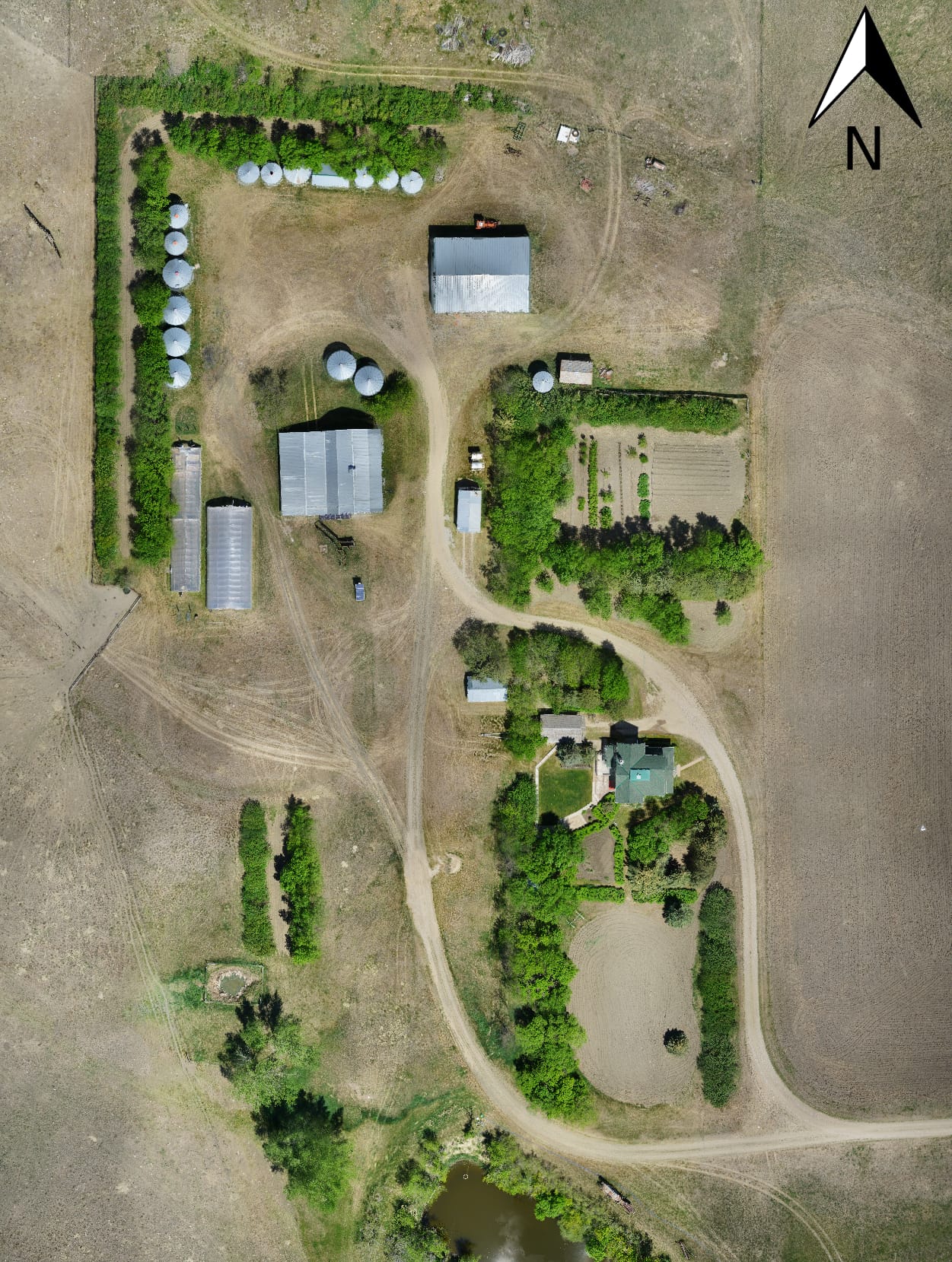
Fig 2.1-1. Demo 1 project area of interest

Attention

The instructions within the following sections were documented using a computer with 32 GB of memory, a NVidia graphics card, and running Windows 10. The tutorial has also been completed (minus the POSPac UAV and Pix4Dmapper processing steps) on a MacBook Pro computer with 16 GB of memory and running Mac OS Mojave. To date, no computers running a Linux OS distro have been tested, though they should work with little to no modifications to the tutorial.

---

2.2 Data Management

It is required to store the files collected by an OpenMMS sensor within an empty directory for each data collection campaign. The OpenMMS sensor firmware automatically increments the names of the collected files for each successive data collection campaign. The names of the collected files make it easy to understand which files relate to the individual data collection campaigns.

Open the directory containing the extracted OpenMMS demo project data. The following figure illustrates the contents of this directory.

Fig 2.2-1. OpenMMS project directory

Inside the flight_data directory, the five OpenMMS datasets, as described in the previous section, are included and represent the data collected within a single data collection campaign (i.e., a single RPAS flight in the case of the Demo Project). The images obtained from the Sony A6000 mapping camera are included within the directory, sony_a6000_images. To decrease the size of the Demo Project Data by approximately 800 MB, a total of 89 images were replaced with solid black images. The need for the images to be replaced with solid black images, rather than just deleting them, will be explained in an upcoming section.

Warning

It is strongly recommended to use the underscore character instead of the space character when naming a directory or file that contains OpenMMS data.

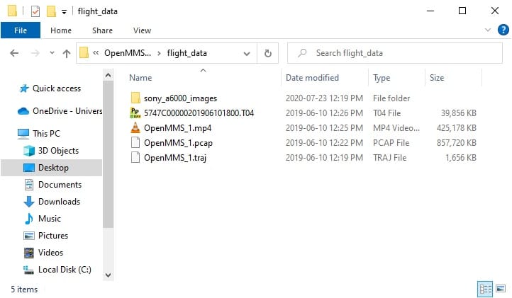
Fig 2.2-2. OpenMMS data collection directory

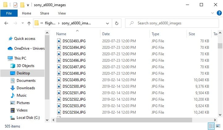
Fig 2.2-3. Sony A6000 images directory

---

2.3 Setup Trigger Files

Attention

The demo project’s lidar data was collected using an OpenMMS sensor with a Velodyne VLP-16 lidar scanner. Therefore, the following documentation discusses and showcases the OpenMMS data processing workflow for sensors with a Velodyne VLP-16.

Be sure to copy the trigger files 1, 3, 4, 5, and 6 that include _vlp16 within their names.

Important

The OpenMMS processing options available within each trigger file will be discussed in full detail within the upcoming section, where the respective trigger file is first used. Full details are not included here.

The next step is to COPY the respective trigger files from the OpenMMS software installation location to the data collection directory. Once inside the data collection directory, the trigger files 7, 8, and 9 need to be MOVED to the sony_a6000_images directory.

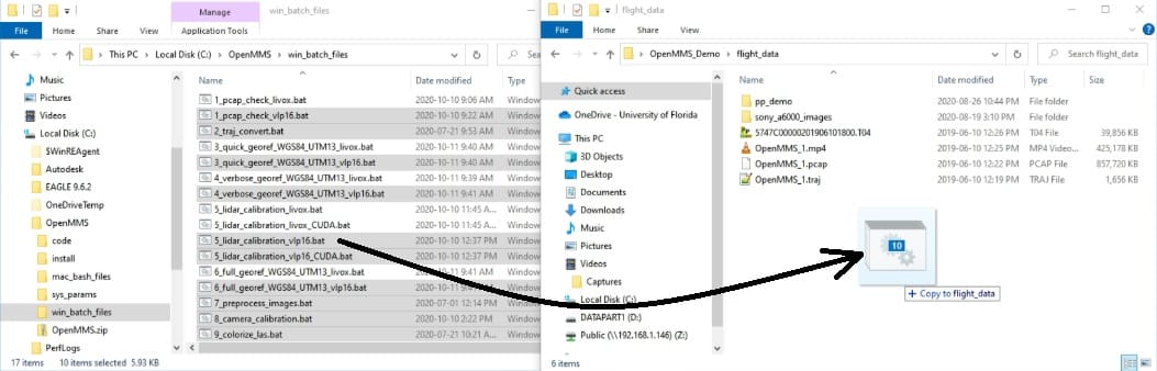
Fig 2.3-1. ALL Windows OS trigger files (.bat) being copied

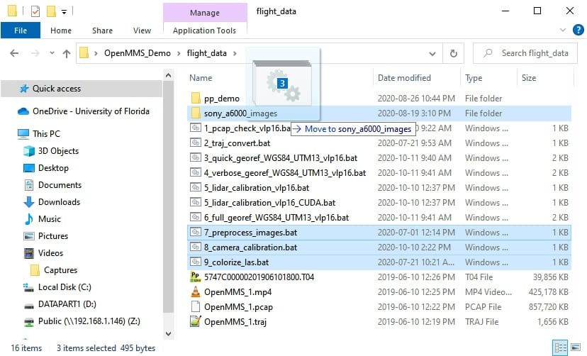
Fig 2.3-2. Mapping camera trigger files being moved

---

2.4 In the Field - Data Processing & QA

The OpenMMS trigger files 1, 2, and 3 are ideally utilized while still in the field immediately after a data collection campaign has finished. The primary goal is to analyze the collected mapping data to ensure that certain characteristics for the point cloud dataset have been achieved (i.e., coverage area, redundancy/overlap, continuous data, etc.).

1_PCAP_CHECK

The 1st trigger file, 1_pcap_check_vlp16, executes the application openmms_pcap_check_vlp16.py. There are NO processing options that can be edited inside this trigger file. Execute the first OpenMMS data processing procedure by double-clicking on the 1_pcap_check_vlp16 file inside the data collection directory. Before execution begins, the 1_pcap_check_vlp16 trigger file searches its directory for files with the .pcap file extension. Only a single .pcap file can be present within the directory for execution to start. Error messages will be reported if no .pcap file exists or if multiple .pcap files exist.

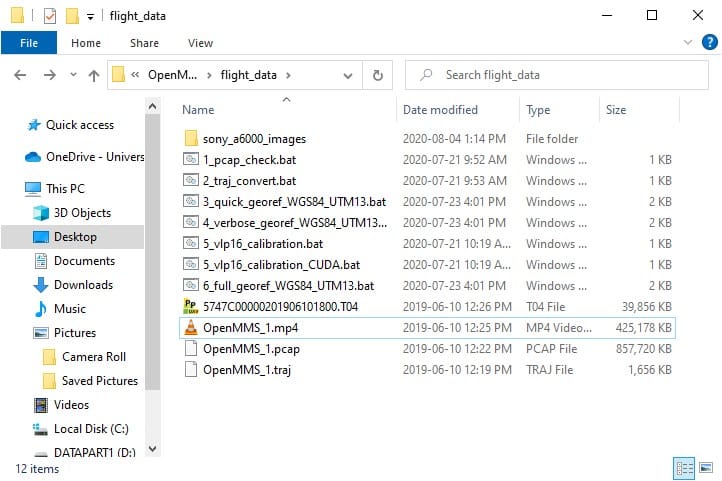
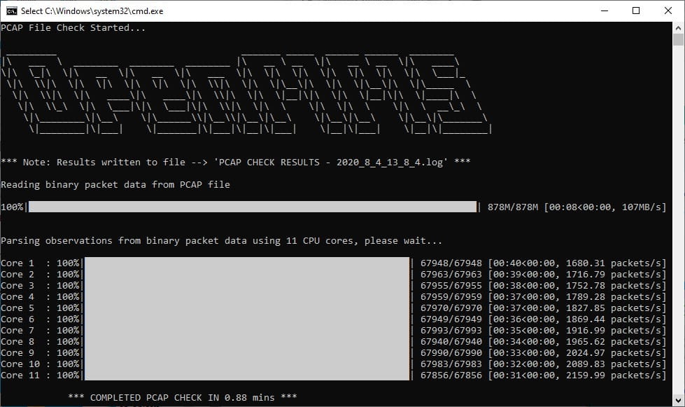
Fig 2.4-1. Directory before executing 1_pcap_check_vlp16	Fig 2.4-2. 1_pcap_check_vlp16 multi-core processing (saved to file)
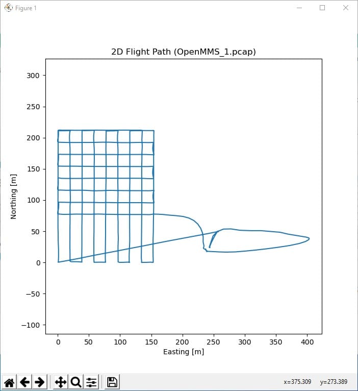
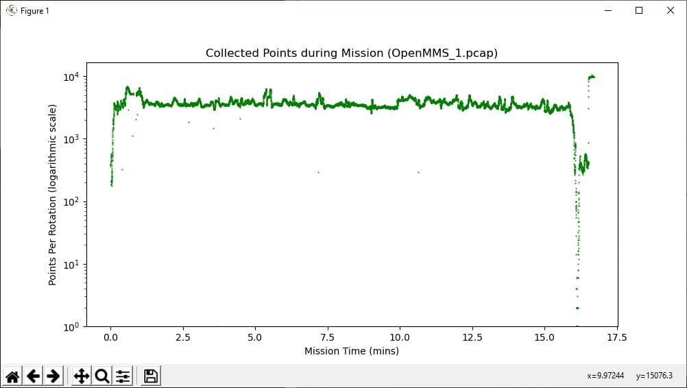
Fig 2.4-3. Trajectory plot (saved to file)	Fig 2.4-4. Collected lidar points during campaign (saved to file)
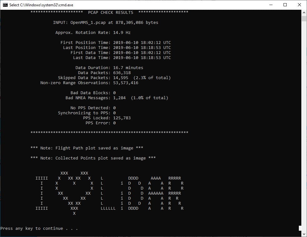
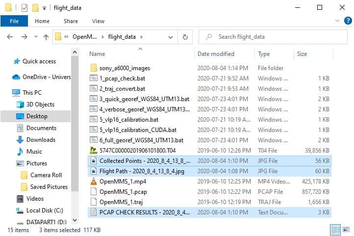
Fig 2.4-5. 1_pcap_check_vlp16 analysis results (saved to file)	Fig 2.4-6. Directory after executing 1_pcap_check_vlp16

1_pcap_check_vlp16 generates three useful quality assurance deliverables about the collected lidar data. Figure 2.4-3 illustrates the plan view plot/map of the lidar sensor during the data collection campaign. The plot shown should agree with the actual ground path the lidar sensor followed. Figure 2.4-4 illustrates the number of valid lidar points (i.e., where the distance observation was not zero) collected for each second of the data collection campaign. Any times when little or no lidar points were being collected will be visible within this plot. Analyzing this plot can lead to improved confidence that adequate and desirable lidar data was collected. Figure 2.4-5 illustrates the valuable quality assurance metadata about the collected lidar data extracted using 1_pcap_check_vlp16. These three deliverables are saved to individual files (2 .jpg and 1 ASCII .log) within the data collection directory, as shown in Figure 2.4-6.

2_TRAJ_CONVERT

The 2nd trigger file, 2_traj_convert, executes the application openmms_traj_convert.py. There are NO processing options that can be edited inside this trigger file. Execute the second OpenMMS data processing procedure by double-clicking on the 2_traj_convert file inside the data collection directory. Before execution begins, the 2_traj_convert trigger file searches its directory for files with the .traj file extension. Only a single .traj file can be present within the directory for execution to start. Error messages will be reported if no .traj file exists or if multiple .traj files exist.

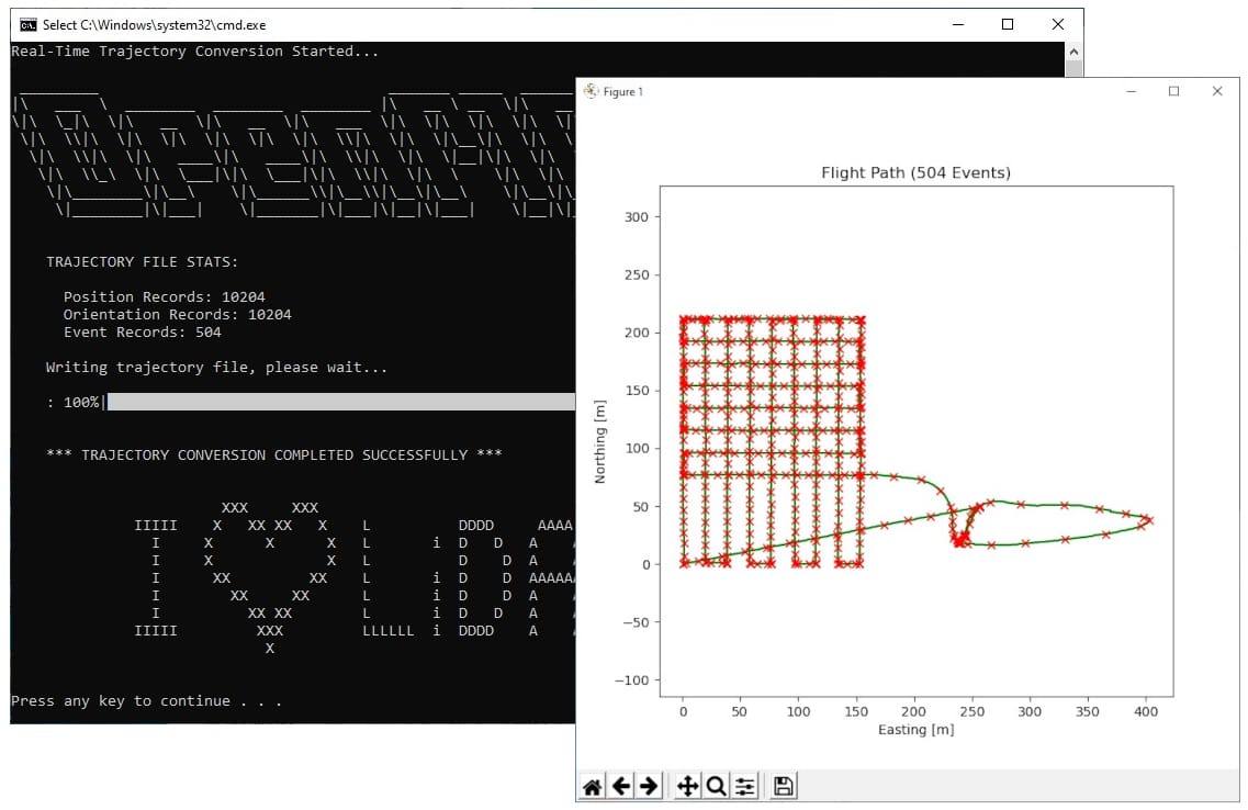
Fig 2.4-7. 2_traj_convert processing and trajectory plot

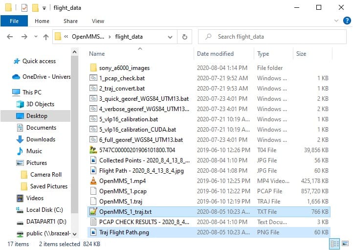
Fig 2.4-8. Directory after executing 2_traj_convert

2_traj_convert generates one useful quality assurance deliverable about the collected Sony A6000 images. Figure 2.4-7 is practically identical to Figure 2.4-3 and illustrates the plan view plot/map of the lidar sensor during the data collection campaign. However, this new plot places X markers at positions where a Sony A6000 camera image was collected. The total number of camera events (i.e., collected images) is listed in the plot’s title and also displayed within the processing results. This plot is saved to a .png file within the data collection directory, as shown in Figure 2.4-8.

Warning

The total number of camera events reported within this step, may be incorrect. Commonly, 1-2 fewer images are reported. Fewer images are reported when the data collection is stopped just before an image was to be taken. Do not be alarmed if the reported total number of camera events does not precisely match the number of images collected by the Sony A6000 camera. It should be within 1 or 2 images.

Lastly, as the name of the 2_traj_convert trigger file implies, the main purpose of this processing step is to convert the raw, real-time trajectory information (i.e., times, positions, and orientations) for the lidar sensor, into a defined format, ASCII-based .txt file. This .txt file is used within the next processing step and provides the capability to produce a georeferenced point cloud dataset from the raw lidar data. The .txt file will have the same filename as the .traj file, as shown in Figure 2.4-8.

3_QUICK_GEOREF

Within the 3rd trigger file, 3_quick_georef…_vlp16, there are eleven processing options that can be edited. Before describing the eleven options, it is important to mention that the OpenMMS trigger files 3, 4, and 6, are virtually identical, with only the processing options stored inside them being different. All three of these trigger files execute the same application, openmms_georeference_vlp16.py. First, open the 3_quick_georef…_vlp16 trigger file using a text editor (do not double click on it). The following figures illustrate the eleven processing options within the trigger file: Windows OS (left) and Mac OS (right).

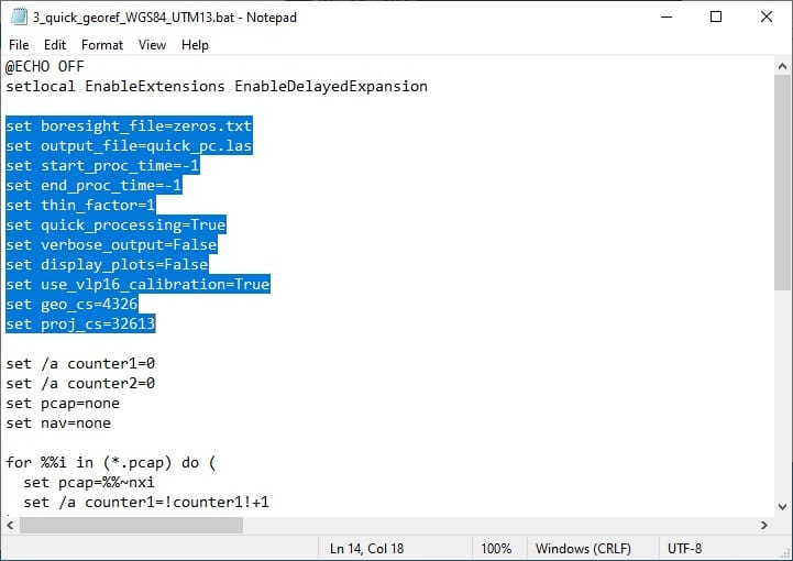
Fig 2.4-9. 3_quick_georef…_vlp16 trigger file (Windows)

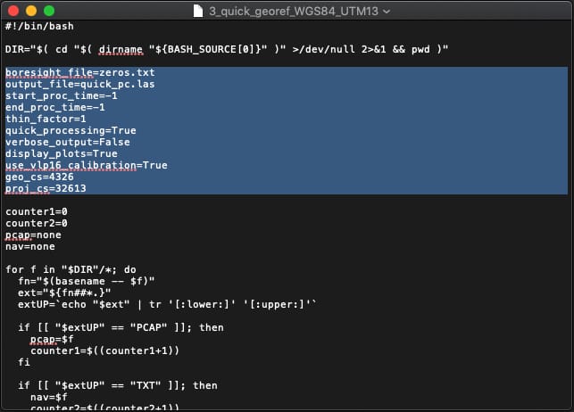
Fig 2.4-10. 3_quick_georef…_vlp16 trigger file (Mac)

The eleven processing options for the openmms_georeference_vlp16.py application are:

1. boresight_file: specifies the ASCII-based file, inside the OpenMMS software installation sys_params subdirectory, that contains the three boresight alignment parameters for the lidar sensor. The default file is zeros.txt. The specified boresight_file can be bypassed if a specially named .bor file is present within the data collection directory (showcased in an upcoming section).

2. output_file: specifies the filename for the point cloud dataset created within the data collection directory. The default filename is quick_pc.las for the 3_quick_georef…_vlp16 trigger file. Supported output file formats include, .las, .laz, and .csv. IMPORTANT NOTE: If a file with this filename already exists within the data collection directory, it will be overwritten without warning!

3. start_proc_time: specifies the starting timestamp for processing data using UTC seconds within the current day. Any data before this timestamp is ignored. This option supports inline addition and subtraction operators (showcased in an upcoming section). The default value is -1, which indicates processing starts at the beginning of the data.

4. end_proc_time: specifies the ending timestamp for processing data using UTC seconds within the current day. Any data after this timestamp is ignored. This option supports inline addition and subtraction operators (showcased in an upcoming section). The default value is -1, which indicates processing stops at the end of the data.

5. thin_factor: specifies a 1/X factor applied to the data (i.e., 2 = 50% of the data will be processed, 10 = 10% of the data will be processed). The data is thinned uniformly across the entire lidar dataset. The default value is 1, which indicates all data is used.

6. quick_processing: specifies if quick processing should be utilized (True) or not (False). Quick processing only processes the lidar data collected from a single laser emitter/detector of the Velodyne VLP-16 sensor. The default value is True for the 3_quick_georef…_vlp16 trigger file.

7. verbose_output: specifies if the generated point cloud dataset should contain the point attributes needed for the boresight calibration processing (showcased in an upcoming section). The default value is False for the 3_quick_georef…_vlp16 trigger file.

8. display_plots: specifies if a data collection analysis plot, similar to Figure 2.4-4, should be displayed after processing has finished. If set to True, an attempt will also be made to load and display the generated point cloud dataset within the CloudCompare application (be sure to use CloudCompare v2.11 or later, or this functionality may not work correctly). The default value is always False. IMPORTANT NOTE: If this option is set to True, a potentially large CloudCompare .bin file also needs to be created inside the data collection directory, thus requiring more computer data storage.

9. use_vlp16_calibration: specifies if a specially named .cal file should be used to define the internal calibration values for the Velodyne VLP-16 lidar sensor. If the file is missing from the data collection directory, this option does not affect the data processing. This option is used to test some experimental processing strategies, currently a work in progress. The default value is True.

10. geo_cs: specifies the EPSG number for the geographic coordinate system (i.e., horizontal datum) of the data. The value of 4326 is for the WGS84 datum. Depending on what part of the World the data is from, this option will most likely need to change.

11. proj_cs: specifies the EPSG number for the desired projected coordinate system (i.e., mapping coordinates) of the data. The value of 32613 is for the WGS84 UTM Zone 13 North. Depending on what part of the World the data is from, this option will most likely need to change.

Tip

It helps to create unique trigger files for specific datum and projection combinations that are frequently used. An example being the 3_quick_georef_WGS84_UTM13_vlp16 trigger file used in this demo project.

Execute the third OpenMMS data processing procedure by double-clicking on the 3_quick_georef_WGS84_UTM13_vlp16 file inside the data collection directory. Before execution begins, the 3_quick_georef_WGS84_UTM13 trigger file searches its directory for files with the .pcap and .txt file extensions. Only a single .pcap file and a single .txt file can be present within the directory for execution to start. Error messages will be reported if no .pcap file or .txt file exists or if multiple .pcap files or .txt files exist.

Tip

It usually always helps to turn on the Eye Dome Lighting (EDL) effect within CloudCompare to visualize the point cloud’s features better.

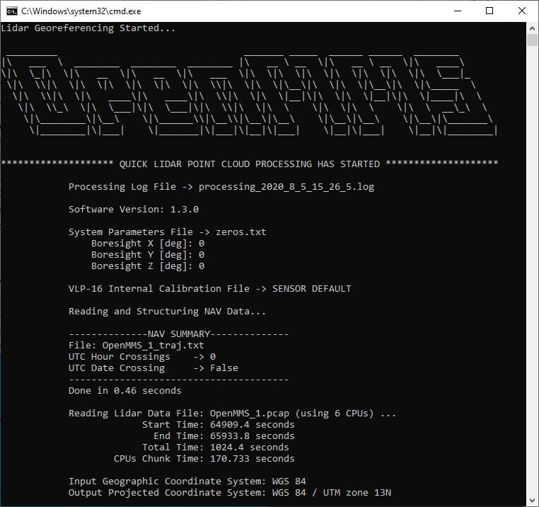
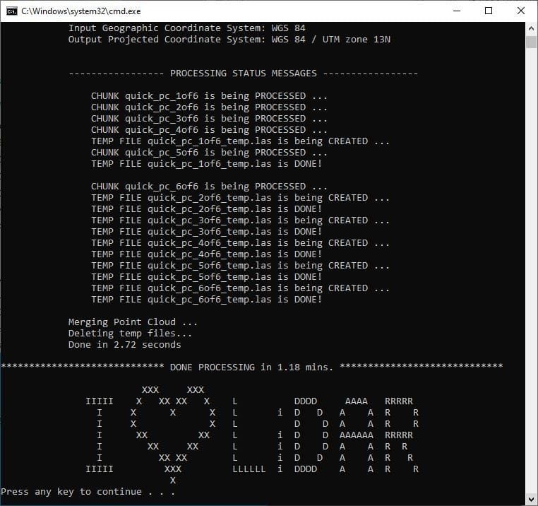
Fig 2.4-11. 3_quick_georef…_vlp16 processing (saved to file)	Fig 2.4-12. 3_quick_georef…_vlp16 processing (multi-core)
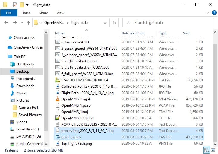
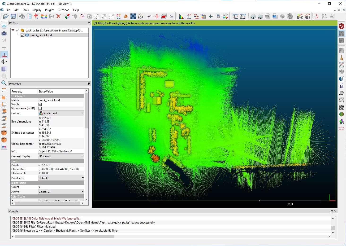
Fig 2.4-13. Directory after executing 3_quick_georef…_vlp16	Fig 2.4-14. quick_pc.las being displayed in CloudCompare (w. EDL)

Important

What this documentation calls attributes, CloudCompare calls Scalar Fields (SF).

The processing information displayed within Figures 2.4-11 and 2.4-12 is saved to an ASCII-based .log file within the data collection directory, as shown in Figure 2.4-13. The primary purpose for 3_quick_georef_WGS84_UTM13_vlp16 is to quickly generate a lower accuracy georeferenced point cloud using the collected data, notice the file quick_pc.las in Figure 2.4-13. Viewing the point cloud’s 3D geometry and attributes within CloudCompare, an understanding of the suitability, or lack thereof, of the collected data can be gained.

Attention

The lower accuracy of the quick_pc.las point cloud is primarily a result of the position and orientation estimates (a.k.a., trajectory data) within the .traj file being calculated using Standard Positioning Service (SPS) GNSS observations. The highest accuracy trajectory data is produced using a Post-Processed procedure, refer to the following figure.

Fig 2.4-15. Applanix APX-18 Performance Specifications (Source: Applanix)

Also, the lidar sensor’s boresight angular misalignment parameters have not yet been estimated. Incorrect values for these parameters can also significantly impact the point cloud’s accuracy. The topic of lidar sensor boresight calibration is discussed in section 2.6.

The accuracy of the point cloud can easily be visualized using CloudCompare (CC). The following video illustrates the steps to perform in CloudCompare to view a cross-section of the point cloud. Notice how the building’s roofline shows several parallel lines of different colored points. The color of the points represents their GpsTime attribute/scalar field (i.e., the different color points were collected at different times during the data collection).

Video 1. Cross section analysis using CC (no audio)

One recommended analysis to perform on the quick_pc.las point cloud, is to determine the start and stop UTC times for the lidar data of interest (reported as seconds within the day). As an example, OpenMMS Hardware - Section 13.9 explained that the Inertial Navigation System (INS) needs to be initialized before starting data collection. Therefore, the lidar data collected during the initialization period is usually of no interest to the project and can be excluded from further processing. Determining the start and stop UTC times does not have to be performed, but it helps to decrease the file sizes of the generated data and the overall processing time. The following video demonstrates the steps to perform in CloudCompare to determine the start and stop UTC times.

Video 2. Start and stop time analysis using CC (no audio)

Warning

For those readers who are new to using CloudCompare, understanding why and when CloudCompare applies shifts to the geometry or attribute data of a point cloud is vital!

The previous video showed that reasonable estimates for a start and stop UTC times were 109.2s and 945.5s, respectively. However, when opening the quick_pc.las file within CloudCompare, the GpsTime attributes for all points, were shifted by a constant amount. Therefore, the estimates of 109.2s and 945.5s are incorrect. To discover the magnitude of the shift applied to the GpsTime attribute, the user must either:

1. read the log messages displayed in CloudCompare’s Console interface and find the message that indicates the shift applied to the Time scalar field (see Figure 2.4-16).

2. assign the Active Scalar Field property to GpsTime and use the Point Picking Tool to select any point on the screen. The coordinates message box that appears will show the actual GpsTime attribute value and the shifted value. The magnitude of the shift can then be calculated as the difference between these two values.

The 2nd approach was demonstrated in the previous video. A screenshot showing the GpsTime attribute within the coordinates message box is shown in Figure 2.4-17. Computing the difference yields a shift value of 64928.01s, which agrees with the reported Console message (of course). Therefore, the correct start and stop UTC times would be, 64928.01+109.2 and 64928.01+945.5, respectively.

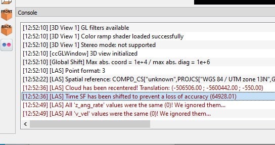
Fig 2.4-16. CC Console showing the applied shift in Time

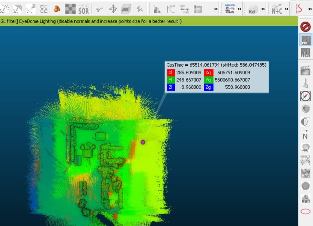
Fig 2.4-17. CC coordinates message box showing Time values

---

2.5 Post-Processed Kinematic (PPK) Trajectory from POSPac UAV

Attention

For those users who do not have access to POSPac UAV software, the two files generated within this section have been included as part of the OpenMMS Demo Project Data. They can be found within the pospac_exports directory.

Note: the event1_eo_5747C00000201906101800_pre_calibration.txt file is the one that is generated within this section.

As discussed in the previous section, the highest accuracy trajectory data is produced using a post-processed procedure. This section demonstrates how to use the Applanix POSPac UAV software to post-process the data in a .T04 file, collected from an Applanix GNSS-INS sensor, along with data in a .T02 file, collected from a Trimble GNSS reference station.

The following summarizes the steps to perform within the POSPac UAV v8.4 SP2 software application:

1. Create a new project using the VLP16 OpenMMS WGS84 UTM EGM96 template.

2. Save the POSPac project within the data collection directory.

3. Import the .T04 file.

4. Modify Project Settings, the GAMS Standard Deviation will ALWAYS need to be manually set to 1cm.

5. Import the .T02 file (RINEX would also work).

6. Modify the reference station coordinates to precise values, including datum and epoch information.

7. Process GNSS data and review results.

8. Process GNSS and Inertial data.

9. Generate QC Report and review results, especially the Total Body Acceleration and Smoothed Performance Metrics.

10. Export the high accuracy trajectory data to a file, using the OpenMMS_Export format.

11. Generate the Exterior Orientation (EO) data for the camera events, using the OpenMMS_Camera format.

12. Determine the first and last camera event numbers that cover the project area of interest.

13. Save the POSPac project again.

The following video demonstrates the previous thirteen steps.

Video 3. POSPac UAV v8.4 SP2 post-processing demonstration (no audio)

There are two files created as part of the POSPac UAV post-processing procedure needed before the OpenMMS data processing workflow can continue. These are Auxiliary Files #5 and #6, as discussed previously in section 2.1. Assuming the reader also named their POSPac project pp_demo, as shown in Video 3, the two required files will be named, export_5747C00000201906101800.txt and event1_eo_5747C00000201906101800.txt. These files can be found in the POSPac project directory’s, Export, and EO subdirectories, respectively. Copy these two files into the data collection directory, as shown in Figure 2.5-1. Then move the event1_eo_574…800.txt file into the sony_a6000_images subdirectory, as shown in Figure 2.5-2.

Lastly, for this demo project, the first camera event of interest was 63, and the last camera event of interest was 478. These event numbers are used within section 2.9 below, see Figure 2.9-1.

Warning

Do NOT change the filenames of two required files created using POSPac UAV! Errors in the upcoming processing steps will result.

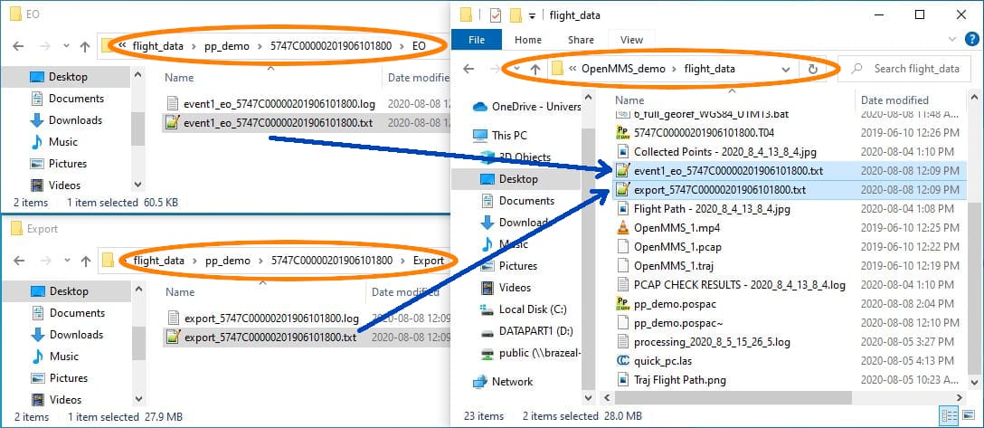
Fig 2.5-1. POSPac UAV generated files copied to data collection directory

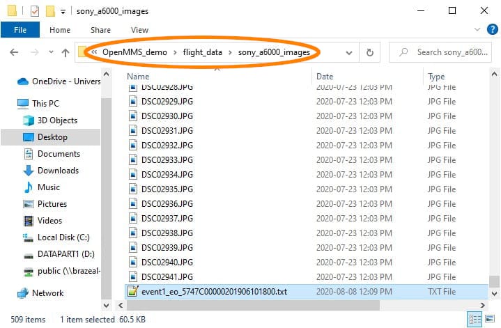
Fig 2.5-2. event1_eo… file moved to sony_a6000_images subdirectory

---

2.6 Lidar Sensor Boresight Calibration

This section presents the second of three calibration procedures that need to be performed on the OpenMMS sensor. Now that the highest accuracy trajectory data has been produced, the lidar sensor’s boresight angular misalignment parameters need to be estimated. There are several published approaches to estimating these parameters. Most, if not all, of the approaches are implemented in-situ rather than in a laboratory environment. An interested reader should have no problem finding vasts amounts of past and present research on this topic. As part of the current OpenMMS data processing workflow, the lidar boresight calibration approach requires the following steps to be performed:

1. Generate a georeferenced point cloud dataset that preserves the lidar observations and high accuracy trajectory parameters for each point.

2. While viewing the georeferenced point cloud using CloudCompare, manually identify unique planar sections (in a wide variety of orientations) and save them to individual files.

3. Execute the 5_lidar_calibration_vlp16 trigger file, which analyzes the individual planar sections and produces a least-squares optimized estimate for the lidar sensor’s boresight angular misalignment parameters. An ASCII-based file will be generated that contains the estimated parameters.

Attention

The OpenMMS lidar boresight calibration approach does NOT require specialized lidar ground targets, or any points, features, or surfaces with known coordinated information, to be successfully utilized. For the best results, an area containing lots of precise planar surfaces (with varying normal directions) should be observed by the lidar sensor multiple times and from multiple different directions.

4_VERBOSE_GEOREF

As previously discussed, the 4th trigger file, 4_verbose_georef…_vlp16, is essentially the same as 3_quick_georef…_vlp16. The only differences are that the output_file, quick_processing, and verbose_output options are set to different default values. To improve the efficiency of the remaining OpenMMS data processing steps, the previously determined start and stop UTC times can be assigned to the start_proc_time and end_proc_time options within the 4_verbose_georef trigger file. Be sure to save the trigger file after editing the processing options.

Tip

Remember, that the start_proc_time and end_proc_time processing options support inline addition and subtraction operators. Therefore, their values can be specified as, 64928.01+109.2 and 64928.01+945.5, respectively. Of course they can also be specified as 65037.21 and 65873.51 if desired.

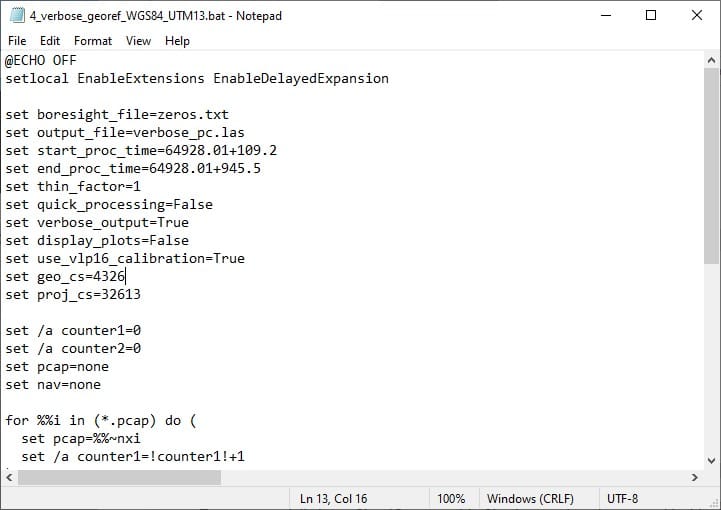
Fig 2.6-1. 4_verbose_georef…_vlp16 file contents

Execute the fourth OpenMMS data processing procedure by double-clicking on the 4_verbose_georef_WGS84_UTM13_vlp16 file inside the data collection directory. Before execution begins, the 4_verbose_georef_WGS84_UTM13_vlp16 trigger file searches its directory for files with the .pcap and .txt file extensions. Only a single .pcap file and a single .txt file can be present within the directory for execution to start. Error messages will be reported if no .pcap file or .txt file exists or if multiple .pcap files or .txt files exist.

Tip

You may receive an error message when attempting to execute the 4_verbose_georef_WGS84_UTM13_vlp16 trigger file. Most likely, this is the result of having two .txt files within the data collection directory. The lower accuracy trajectory file, OpenMMS_1_traj.txt is no longer needed and must be removed or renamed with a different file extension for the execution to start.

The files generated from the execution of the 4_verbose_georef…_vlp16 trigger file are created in the data collection directory and include, an ASCII-based .log file, the georeferenced point cloud with the verbose attributes (named verbose_pc.las within this demo project), and a new subdirectory named calibration1, see Figure 2.6-4. Within the calibration1 directory, there will be a single .csv file named verbose_offsets.csv. Do not delete or rename this .csv file or errors will occur within upcoming processing steps! Lastly, move the 5_lidar_calibration_vlp16 Trigger File(s) from the data collection directory into the calibration1 subdirectory, see Figure 2.6-5.

Attention

If a subdirectory with the name calibration1 already exists, the 4_verbose_georef…_vlp16 execution will NOT overwrite the subdirectory. Instead, the new subdirectory will be named calibration2, and it will need to be used within the upcoming processing steps. This logic holds for all subdirectories named calibration followed by a number.

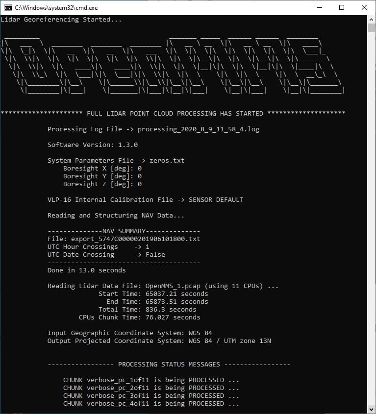
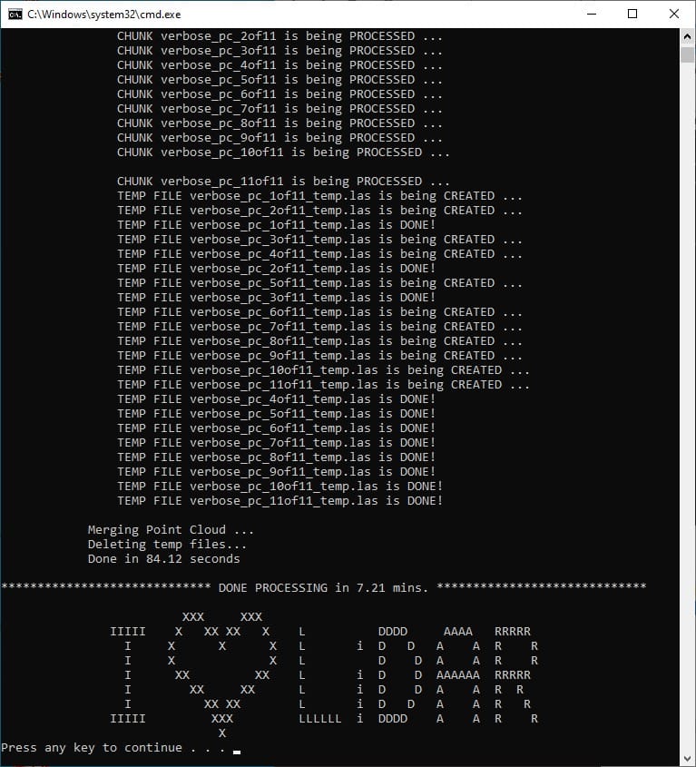
Fig 2.6-2. 4_verbose_georef…_vlp16 processing (saved to file)	Fig 2.6-3. 4_verbose_georef…_vlp16 processing (multi-core)
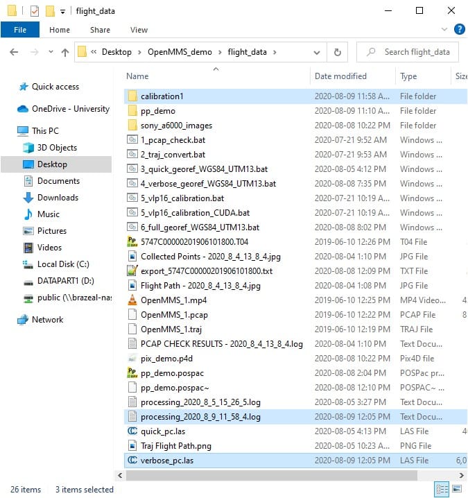
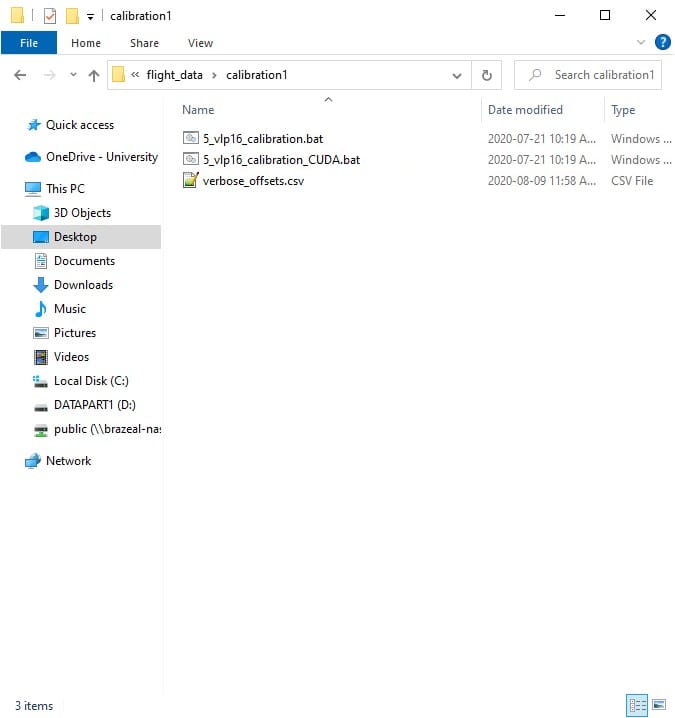
Fig 2.6-4. Directory after executing 4_verbose_georef…_vlp16	Fig 2.6-5. Move 5_lidar_calibration_vlp16 trigger file(s) to calibration directory

Next, open the verbose_pc.las point cloud dataset within the CloudCompare software application. Manually identify, select, and clip out planar sections from the point cloud, see Figure 2.6-6 for instructions on how to clip out a smaller section from the overall point cloud. The individual clipped sections should be examined to ensure that the selected points all represent the same planar feature, see Figures 2.6-9 to 2.6-11. Lastly, the planar sections need to be saved to individual ASCII-based .txt files within the aforementioned calibration1 subdirectory, see Figures 2.6-12 and 2.6-13. As previously mentioned, a variety of planar sections with different orientations is ideal.

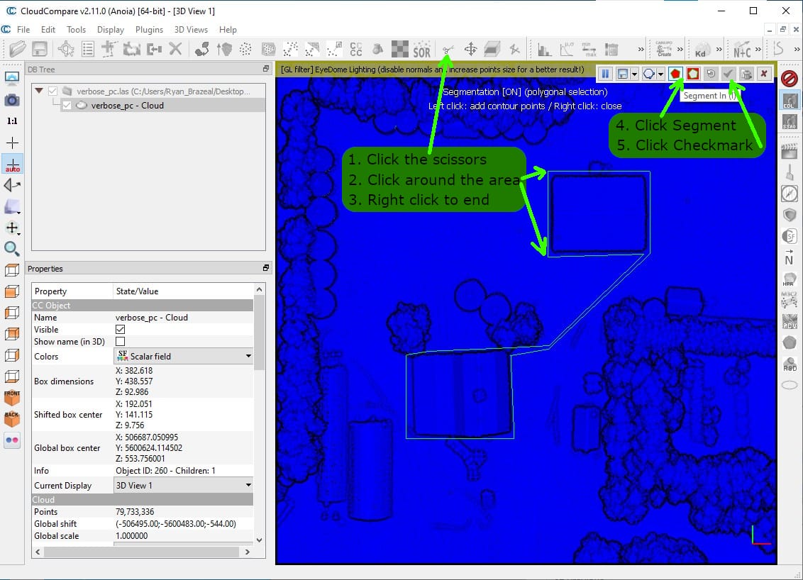
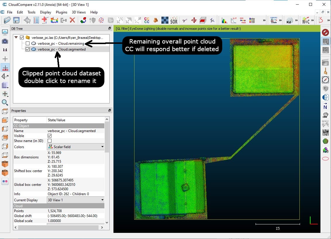
Fig 2.6-6. verbose_pc.las in CloudCompare (79.7M pts.)	Fig 2.6-7. Isolate buildings with planar features (only 1.5M pts.)
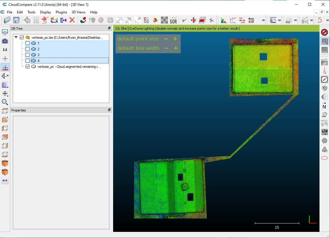
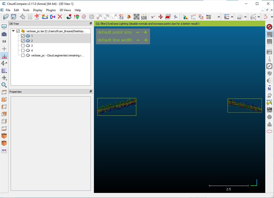
Fig 2.6-8. Clipping 4 small planar sections from the roofs	Fig 2.6-9. Check all clipped points represent the planar sections
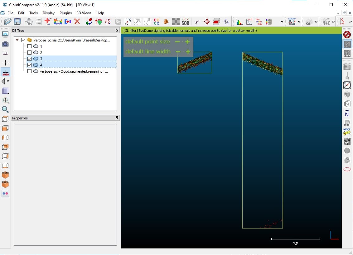
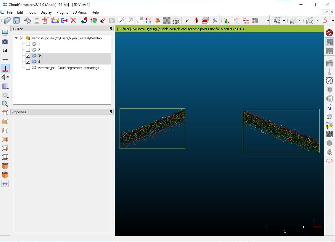
Fig 2.6-10. Some points in planar section 3 are obviously incorrect	Fig 2.6-11. Planar section 3 is clipped again to remove incorrect points
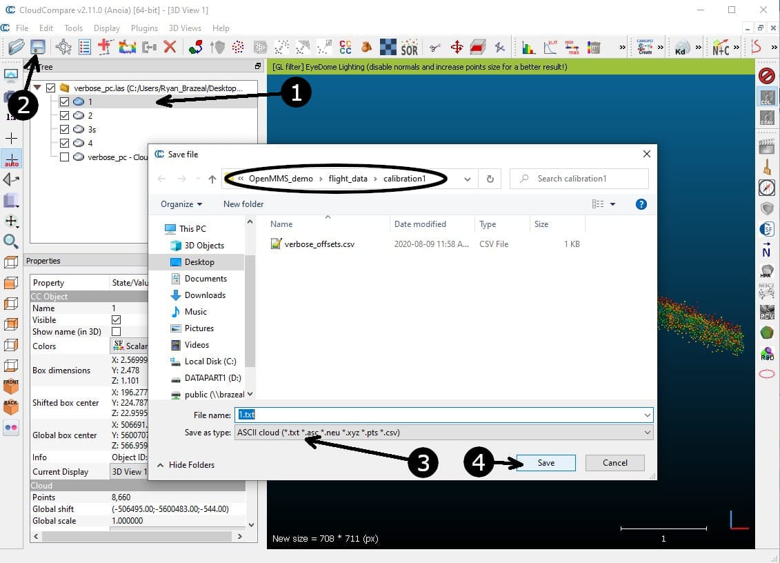
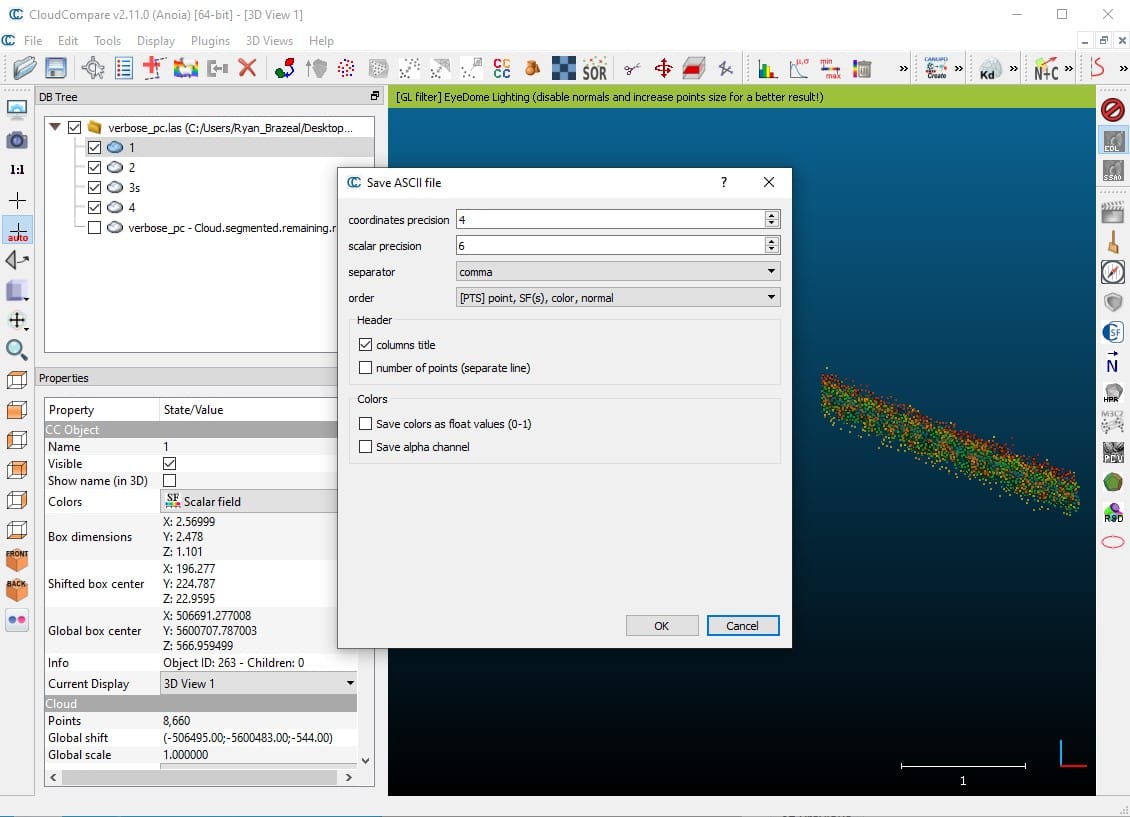
Fig 2.6-12. Select single clipped section and save it as a .txt ASCII cloud	Fig 2.6-13. CC ASCII cloud options (must use exactly as shown)

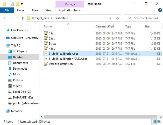
Fig 2.6-14. The calibration1 subdirectory after clipping planar sections

5_LIDAR_CALIBRATION

Within the 5th trigger file, 5_lidar_calibration_vlp16, there are three EXPERIMENTAL processing options that can be edited. This trigger file executes the application, openmms_lidar_calibration_vlp16.py. To begin, open the 5_lidar_calibration_vlp16 file using a text editor (do not double click on it). The following figure illustrates the three experimental processing options within the trigger file on Windows OS.

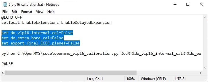
Fig 2.6-15. 5_lidar_calibration_vlp16 trigger file contents (Windows)

The three experimental processing options for the openmms_lidar_calibration_vlp16.py application are:

1. do_vlp16_internal_cal: after the boresight parameters have been estimated (and now held fixed), this option specifies if the planar sections should again be analyzed, but now to estimate the forty-eight internal calibration parameters of a Velodyne VLP-16 lidar sensor. With the forty-eight parameters being, the range scale factor, horizontal angle offset, and vertical angle offset for each of the sixteen individual laser emitter/detector components (3 x 16 = 48). The default value is False. If this option is set to True, an additional ASCII-based .cal file will be created in the calibration1 subdirectory. This file is the one that is referenced in the processing option use_vlp16_calibration within the 3_QUICK_GEOREF section above.

2. do_extra_bore_cal: specifies if the boresight parameters should be estimated/checked after the internal VLP-16 calibration is performed. The default value is False. This option has no effect if the do_vlp16_internal_cal option is set to False.

3. export_final_ECEF_planes: specifies if the input planar section point clouds should be exported after being recomputed with the estimated boresight parameters being applied. The exported planar sections are within an Earth-Centered Earth-Fixed (ECEF) reference frame. The default value is False.

Warning

These experimental processing options should all be set to False to ensure that the OpenMMS data processing produces the best possible results. These experimental features are very much a work in progress!

Execute the fifth OpenMMS data processing procedure by double-clicking on the 5_lidar_calibration_vlp16 file that is inside the calibration1 subdirectory (or the 5_lidar_calibration_vlp16_CUDA file, if the user is using a Windows OS based computer that has an NVidia CUDA capable Graphics Card). The application attempts to read the contents of all the .txt files within the calibration1 subdirectory as individual point clouds representing unique planar sections. Figure 2.6-16 illustrates the application’s basic summary information, including a tabular distribution of the lidar observations collected by the individual laser emitter/detector components. The benefit of using NVidia CUDA GPU processing is evident when comparing Figures 2.6-17 and 2.6-18. As mentioned, a current development effort is underway to utilize NVidia CUDA GPU processing within as many OpenMMS applications as possible.

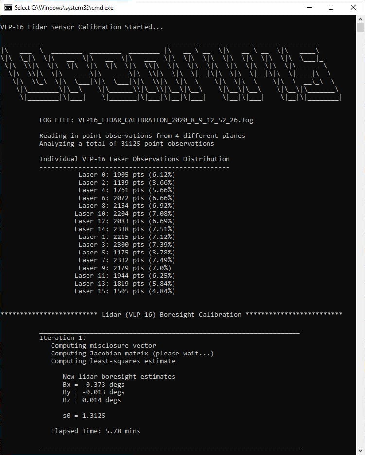
Fig 2.6-16. OpenMMS Lidar Calibration (VLP-16) summary information (saved to file)

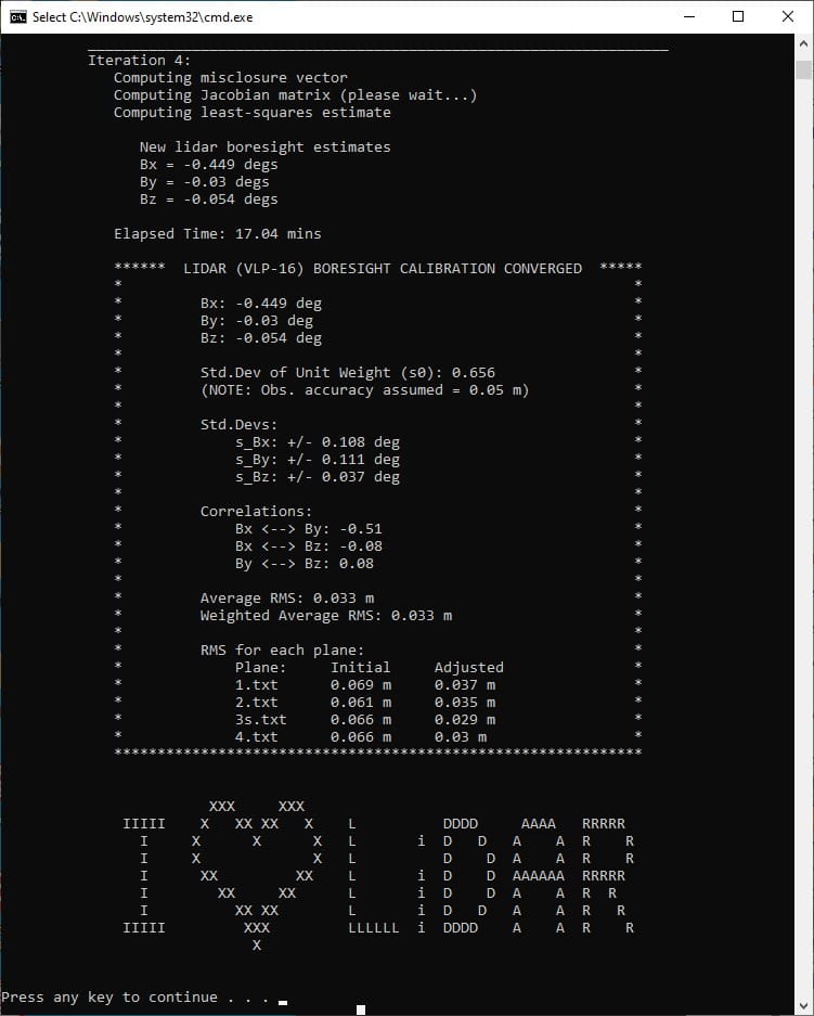
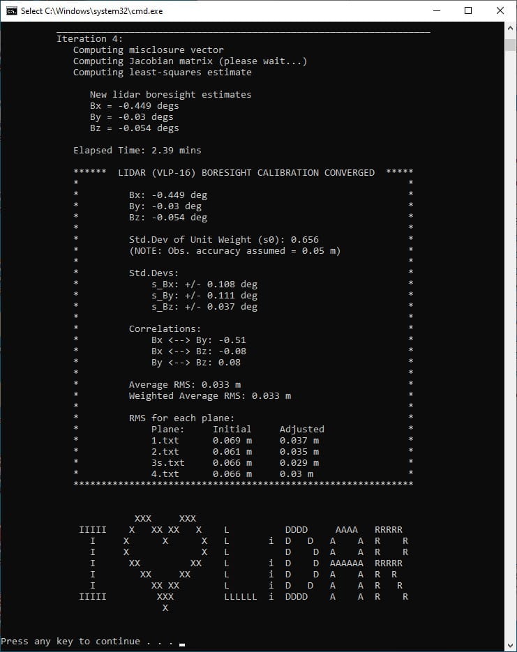
Fig 2.6-17. 5_lidar_calibration_vlp16 results (elapsed time: 17 mins)	Fig 2.6-18. 5_lidar_calibration_vlp16_CUDA results (elapsed time: 2.4 mins)
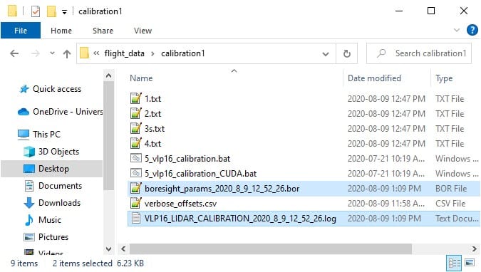
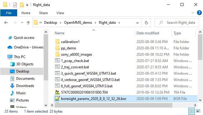
Fig 2.6-19. The calibration1 subdirectory after 5_lidar_calibration_vlp16	Fig 2.6-20. Lidar boresight estimates .bor file copied to DC dir.

The files generated from the execution of the 5_lidar_calbration_vlp16 trigger file are created in the calibration1 subdirectory and include, an ASCII-based .log file, and an ASCII-based .bor file. The .bor file contains the estimates for the lidar sensor’s boresight angular misalignment parameters. The .bor file will be used within the final lidar georeferencing process, by either:

1. Copying the .bor file into the data collection directory for the current demo project, and all future data collection directories for other projects using the same OpenMMS sensor (assuming the lidar boresight estimates remain constant with time). The openmms_georeference_vlp16.py application automatically looks for specially named .bor files upon execution and will use the newest file if more than one is found. If a .bor file is found within the data collection directory, it will be used instead of the file specified in the boresight_file processing option.

2. Copying the .bor file into the OpenMMS software installation sys_params subdirectory, and then editing the boresight_file processing option in the trigger files 3, 4, and 6 within the OpenMMS software installation win_batch_files and mac_bash_files subdirectories. Using this approach, all future processing projects will use these edited trigger files, and therefore will use the .bor file.

For this demo project, the .bor file simply needs to be copied to the data collection directory, as shown in Figure 2.6-20.

Warning

Do not change the filename for the generated .bor file, or the lidar boresight estimates may not be applied within the georeferencing processes.

---

2.7 Final Point Cloud Processing & Filtering

With the lidar sensor’s boresight angular misalignment parameters now estimated, the final georeferenced point cloud dataset for the demo project can be generated. The final point cloud is generated using the lidar data, the high accuracy trajectory data, and the lidar boresight estimates. The final processing is executed using the 6_full_georef…_vlp16 trigger file.

6_FULL_GEOREF

As previously discussed, the 6th trigger file, 6_full_georef…_vlp16, is virtually the same as 3_quick_georef…_vlp16 and 4_verbose_georef…_vlp16. The only differences are the values set for some of the processing options. To improve the efficiency of the remaining OpenMMS data processing steps, the previously determined start and stop UTC times can be assigned to the start_proc_time and end_proc_time options within the 6_full_georef…_vlp16 trigger file. Be sure to save the file after editing the processing options.

Tip

Remember that the start_proc_time and end_proc_time processing options support inline addition and subtraction operators. Therefore, their values can be specified as, 64928.01+109.2 and 64928.01+945.5, respectively. Of course they can also be specified as 65037.21 and 65873.51 if desired.

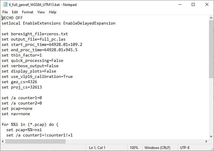
Fig 2.7-1. 6_full_georef…_vlp16 file contents

Execute the sixth OpenMMS data processing procedure by double-clicking on the 6_full_georef_WGS84_UTM13_vlp16 file inside the data collection directory. Before execution begins, the 6_full_georef_WGS84_UTM13_vlp16 trigger file searches its directory for files with the .pcap and .txt file extensions. Only a single .pcap file and a single .txt file can be present within the directory for execution to start. Error messages will be reported if no .pcap file or .txt file exists or if multiple .pcap files or .txt files exist.

The files generated from the execution of the 6_full_georef…_vlp16 trigger file are created in the data collection directory and include, an ASCII-based .log file and the final georeferenced point cloud (named full_pc.las within this demo project), see Figure 2.7-3.

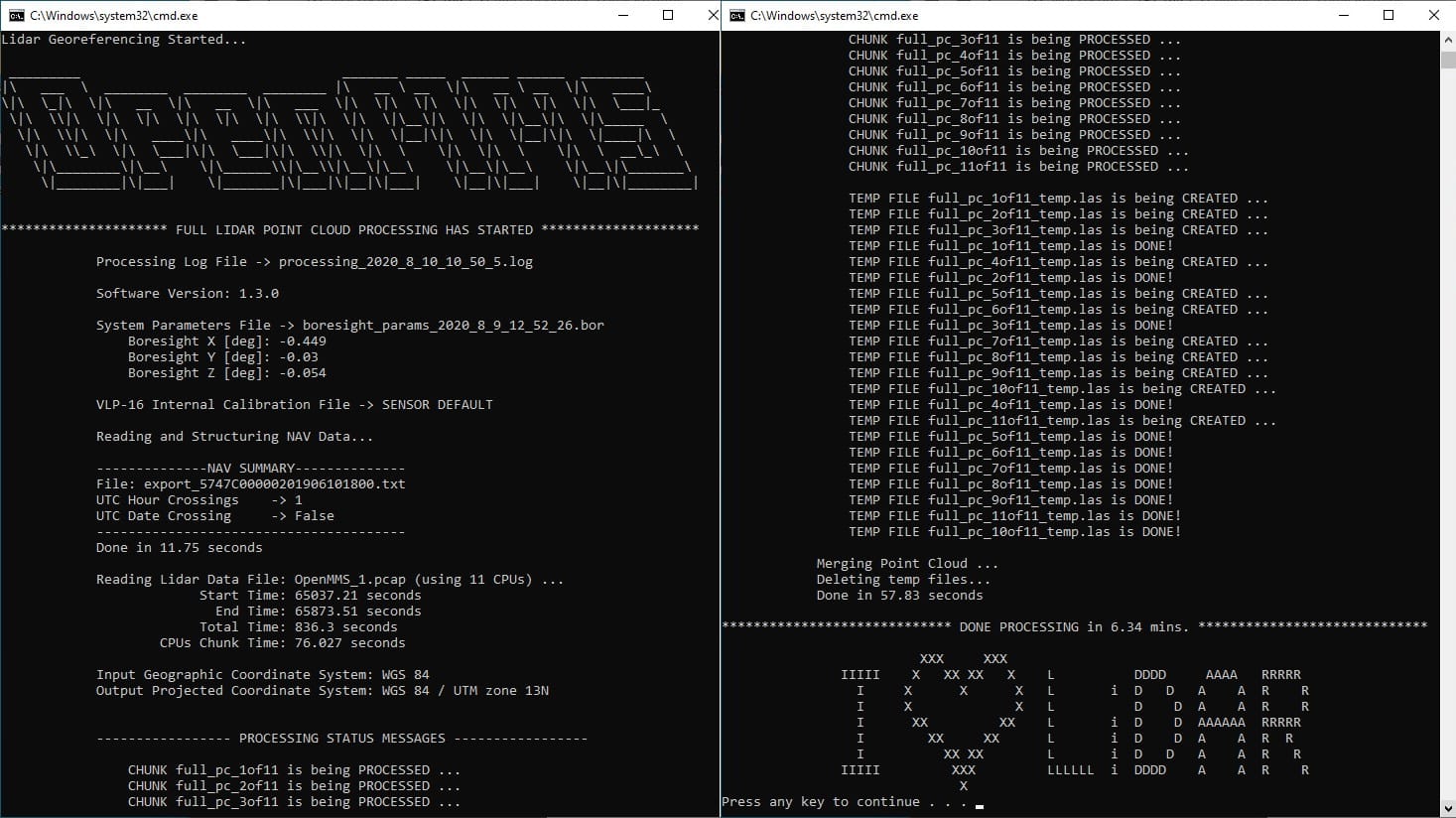
Fig 2.7-2. 6_full_georef…_vlp16 processing results (saved to file)

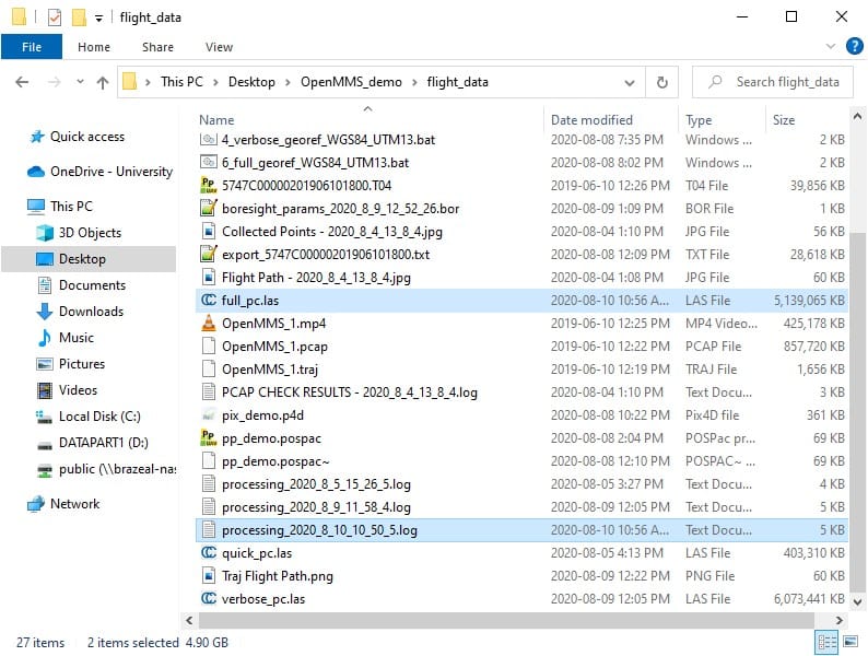
Fig 2.7-3. Directory after executing 6_full_georef…_vlp16

The last step in generating the final georeferenced point cloud is to open the full_pc.las file within CloudCompare and remove the unwanted/unnecessary points by filtering based on the point attributes. The following list discusses the ten OpenMMS Extended LAS attributes followed by the three Standard LAS attributes present within the quick and full OpenMMS generated point clouds.

1. scan_azi defines the azimuth angle of the point (within the scanner’s coordinate system). Refer to Figure 8.7-3 in the OpenMMS Hardware documentation for clarification on the scan_azi values. By filtering based on this attribute, the Field of View (FOV) values configured for the Velodyne VLP-16 sensor can be reduced (but not increased) after data collection. Units are decimal degrees.

2. delta_roll defines the change in the roll orientation angle of the point, with respect to the previously data packet of observed points. This attribute is a remnant of a previous georeferencing approach and no longer plays a vital role in filtering the final point cloud. However, it can still be used to filter out point data observed when the sensor was experiencing quickly changing roll orientation angles during data collection. Units are decimal degrees per second.

3. z_ang_rate defines the lidar sensor’s rate of angular change around the Z axis of the vehicle body frame (i.e., an approximate to the rate of angular change around the direction of the vertical). Similar in usage to the delta_roll attribute, where filtering based on this attribute can eliminate points observed when the sensor was experiencing quickly changing ~heading orientation angles during data collection. Units are decimal degrees per second.

4. v_vel defines the vertical velocity of the sensor when the point was observed. For OpenMMS data collection campaigns from RPAS platforms, this attribute can be used to filter out the take-off and landing time periods (assuming the vertical velocity of the sensor is fairly constant during data collection). Units are meters per second.

5. h_vel defines the horizontal speed of the sensor when the point was observed. This attribute can be used to filter out periods when the sensor was not moving forward, backwards, left, or right, or when the sensor was only rotating (e.g., during stationary turns at the end of RPAS flight lines). Units are meters per second.

6. total_accel defines the absolute value of the total acceleration of the sensor when the point was observed. This atrribute can be used to filter out periods when the sensor was experiencing higher vibrations. Units are g’s (i.e., 1 g = 9.81 m/s^2)

7. scan_num defines a unique ID number for the single rotation of the Velodyne VLP-16 sensor when the point was observed. This attribute will appear to have X distinct chunks of values, where X represents the number of CPU processors used during the 6_full_georef georeferencing. Each chunk of numbers is incremented by 100,000 to crudely avoid using duplicate ID numbers. This attribute is intended for future development of Simultaneous Localization and Mapping (SLAM) techniques within the georeferencing process and the lidar boresight estimation process. It is a unitless attribute.

8. heading defines the direction of the sensor when the point was observed. It is important to remember that the sensor is orientated with respect to the vehicle body, such that the side of the sensor where the Sony A6000 camera is mounted (referred to as the Back Face in Hardware documentation), is aligned with the forward/front direction of vehicle body (see section 13.1 in the OpenMMS Hardware documentation for complete details). As a result, the heading attribute is defined as the clockwise angle around the vertical direction with 0 degrees representing the geographical East direction. Units are decimal degrees.

9. laser_num defines the individual laser emitter/detector component within the Velodyne VLP-16 sensor that observed the point. The attribute values represent the fixed vertical angle of the observing laser (within the scanner’s coordinate system) and are the odd integer numbers within the range of -15 to 15 inclusive. This attribute can be used to filter out any specific observing laser(s) within the VLP-16. Units are integer degrees.

10. range defines the line of sight distance observed from the Velodyne VLP-16 sensor to the point. Many errors are directly proportional to the observed range, so filtering the point cloud based on this attribute can better control the point cloud’s precision. Units are meters.

11. ReturnNumber defines if the point was the first (value = 1) or second (value = 2) observed feature from a single pulse of an observing laser. It is a unitless attribute.

12. GpsTime defines the precise time the point was observed. Units are seconds within the current UTC day. For the special case when the data collection campaign spans across multiple UTC days, the attribute values for the respective points will be greater than 86,400 (i.e., the number of seconds within one day).

13. Intensity defines an 8 bit (0-255) number representing the returned ‘signal strength’ of the transmitted laser pulse. Following the Velodyne VLP-16 documentation, attribute values in the range of 0-100 indicate the observed point is from a non-retroreflective surface, where values >100-255 indicate the observed point is from a retroreflective surface. By filtering based on this attribute, a significant amount of obviously erroneous points can often be removed. It is a unitless attribute.

The combination of attributes to use to filter the full point cloud and create the final point cloud are not absolute. The attributes that best filter the full point cloud in the desired way(s) are dependent on many different factors. The user is strongly encouraged to experiment with filtering using the different attributes, to better understand the impacts each has. The following figures demonstrate the full point cloud being filtered based on h_vel, and then the results being further filtered by range. Once the filtering has been completed, the resulting point cloud needs to be saved from CC to a file within the data collection directory. For the purposes of this tutorial, the resulting point cloud needs to be saved using the filename filtered.las

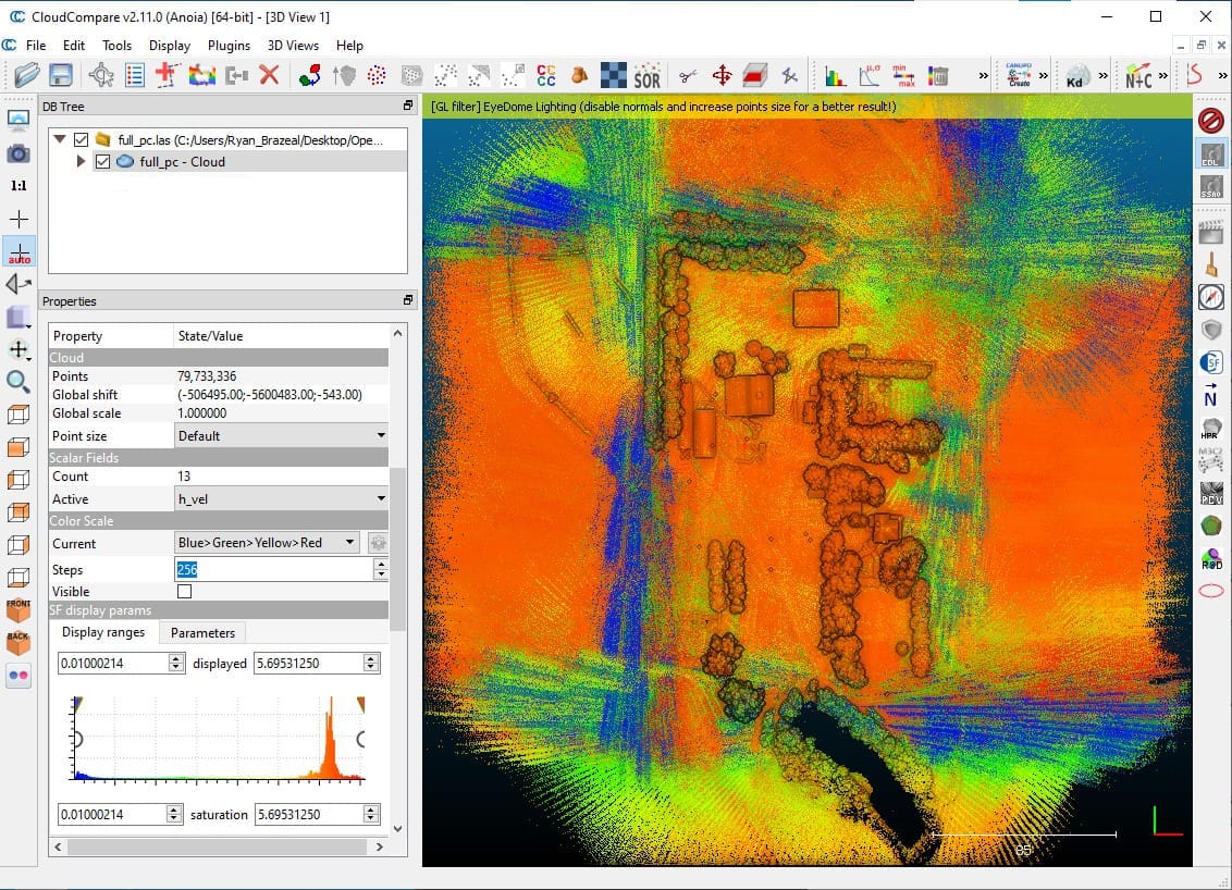
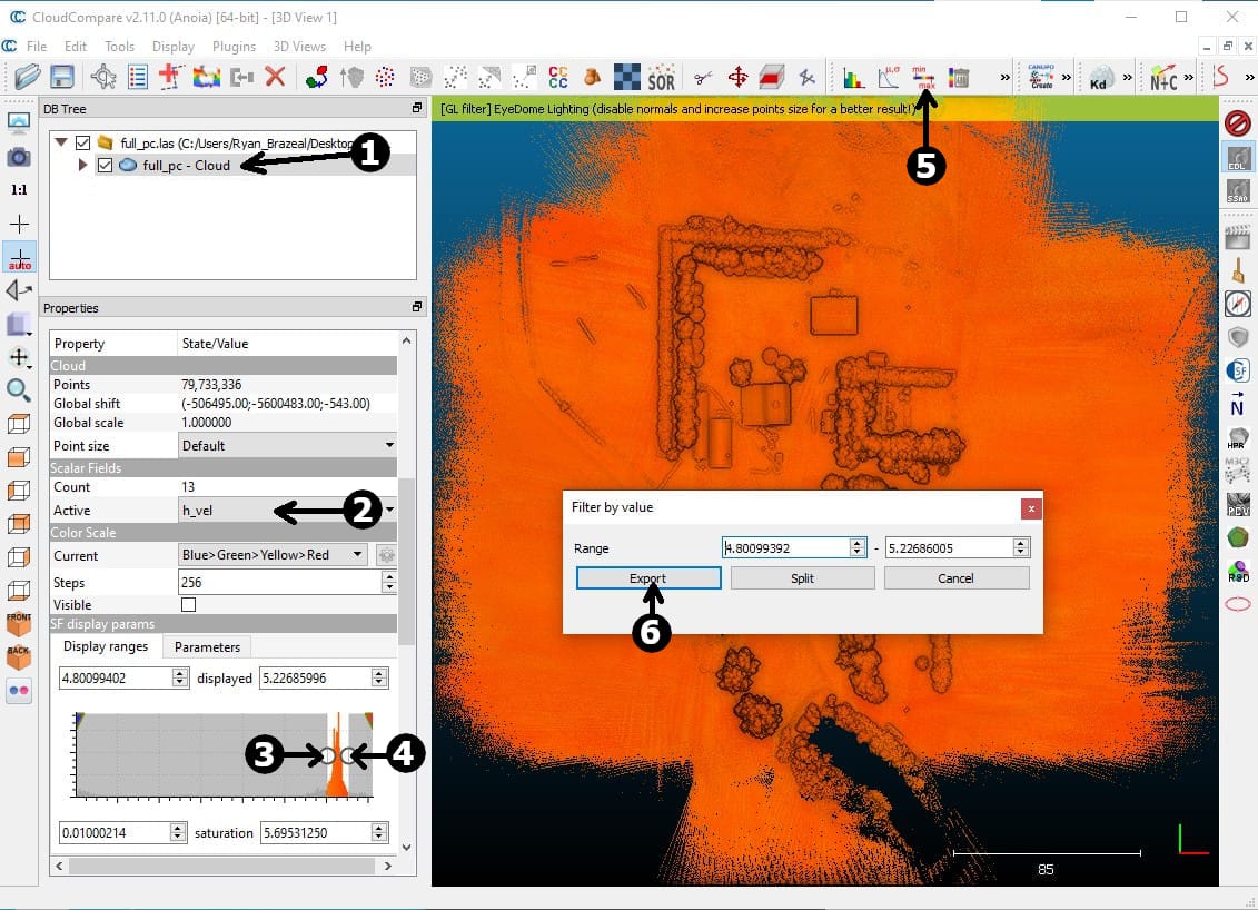
Fig 2.7-4. full_pc.las colored by h_vel values in CC (79.7M pts.)	Fig 2.7-5. Steps to generate a filtered point cloud in CC
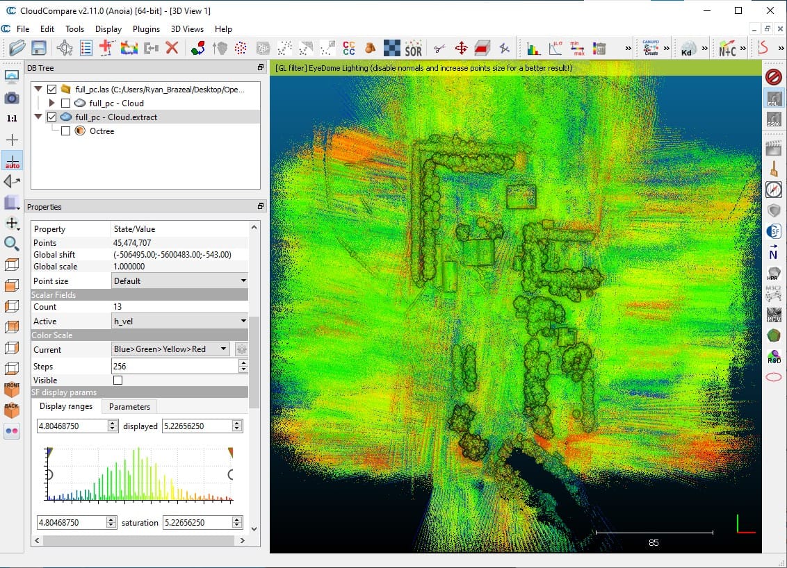
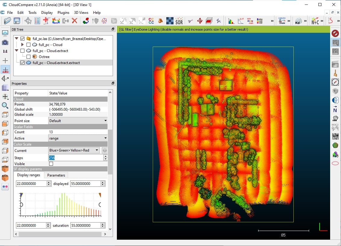
Fig 2.7-6. Results of filtering by h_vel (45.4M pts.)	Fig 2.7-7. Results further filtered by range (34.7M pts.)
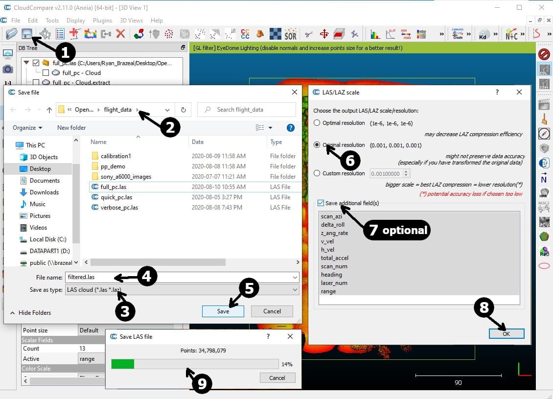
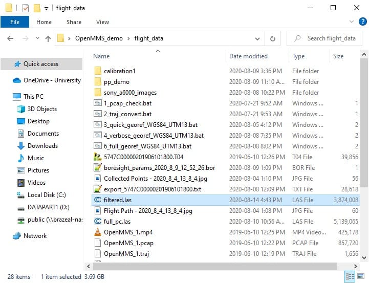
Fig 2.7-8. Save filtered point cloud to filtered.las	Fig 2.7-9. Directory after saving the filtered point cloud

---

2.8 Point Cloud Quality Assurance

The georeferenced point cloud is now in its final state (geometrically speaking). Now is the opportune time to visually and quantitatively assess the spatial accuracy and precision of the OpenMMS point cloud. Begin by opening the filtered point cloud within CloudCompare. Next, import the auxiliary dataset #4 (NEH_ground_pts.csv file found within the Demo Project’s gnss_reference_data subdirectory) into CloudCompare. NOTE: the coordinate order for the file NEH_ground_pts.csv is Y, X, Z.

While holding the CTRL key, click the filtered and NEH_ground_pts point clouds within the DB Tree List in CloudCompare. Then, click on the Compute cloud/cloud distance button in the Main tools toolbar. Follow the steps and enter the processing options, as shown in Figure 2.8-2. At this point, the slope distance and the distances in the X, Y, and Z directions between each RTK ground point and their closest respective point within the georeferenced point cloud have been computed. For QA purposes, we are interested in examining the Z distances (i.e., elevation differences) for the RTK points and their closest point cloud estimates. Follow the steps, as illustrated in Figure 2.8-3, to isolate the RTK points and have them colored according to their respective elevation differences. Examine the spatial distribution of the elevation differences across the project area. As a final step, a Gaussian distribution can be best-fit to the sample of elevation differences to visually see if the sample is exhibiting the behavior of a random dataset. The fitted distribution will also report a mean and standard deviation estimate (which are meaningless unless the sample fits a Gaussian distribution).

Attention

It is important to remember, that this analysis is comparing discrete RTK observed points, that were manually identified by a human operator as being on the ground, against points observed by a lidar sensor, that was attached to an RPAS vehicle flying 40 m above the ground and moving at 5 m/s.

Tip

From experience, vegetated areas within the georeferenced point cloud (i.e., a digital surface model - DSM) will likely report more considerable elevation differences to RTK ground points collected within these areas. For best results, the georeferenced DSM point cloud should be further processed to estimate a digital terrain model (DTM) for the project area, and then the DTM should be compared against the RTK ground points. Producing a DTM from a DSM is outside the scope of this documentation.

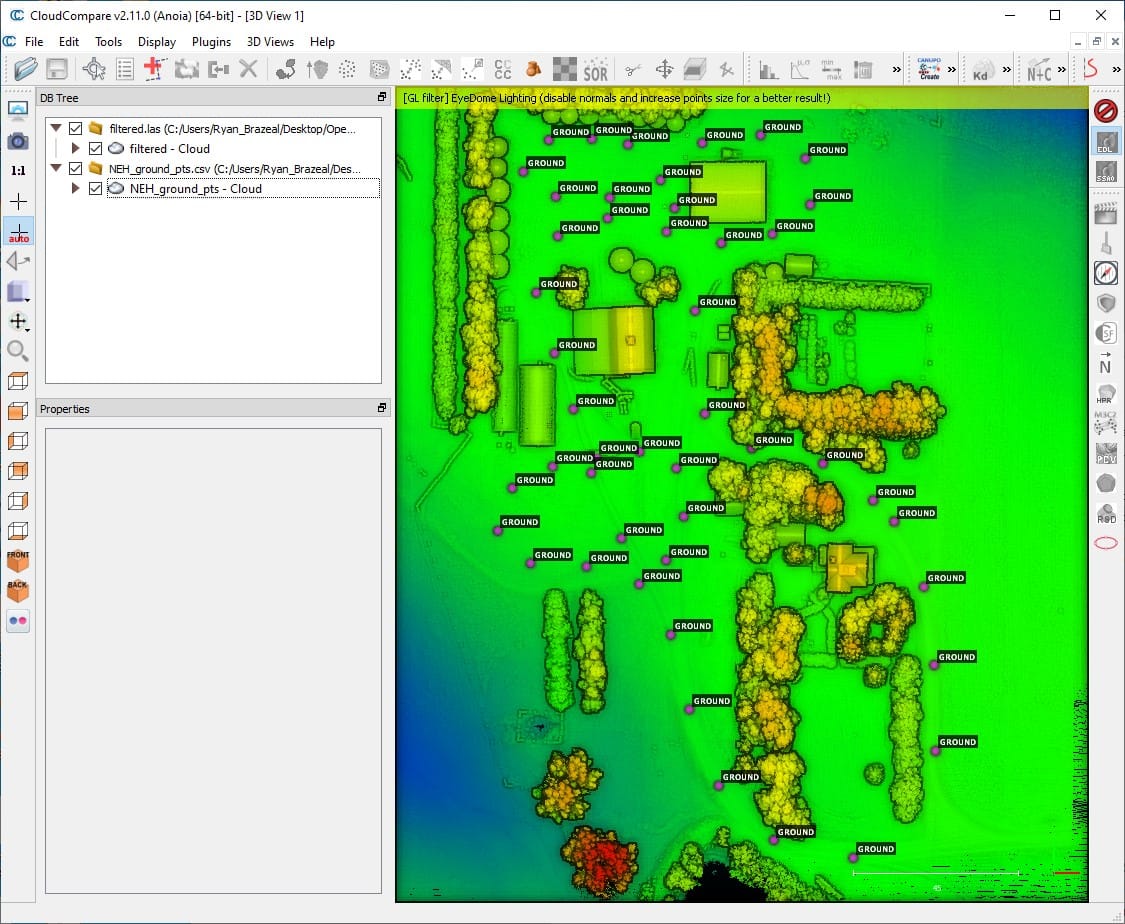
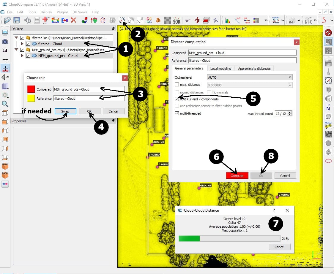
Fig 2.8-1. Filtered point cloud and ground points in CloudCompare	Fig 2.8-2. Steps to perform cloud to cloud comparison in CloudCompare
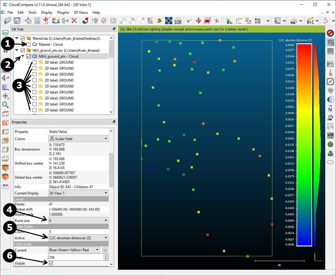
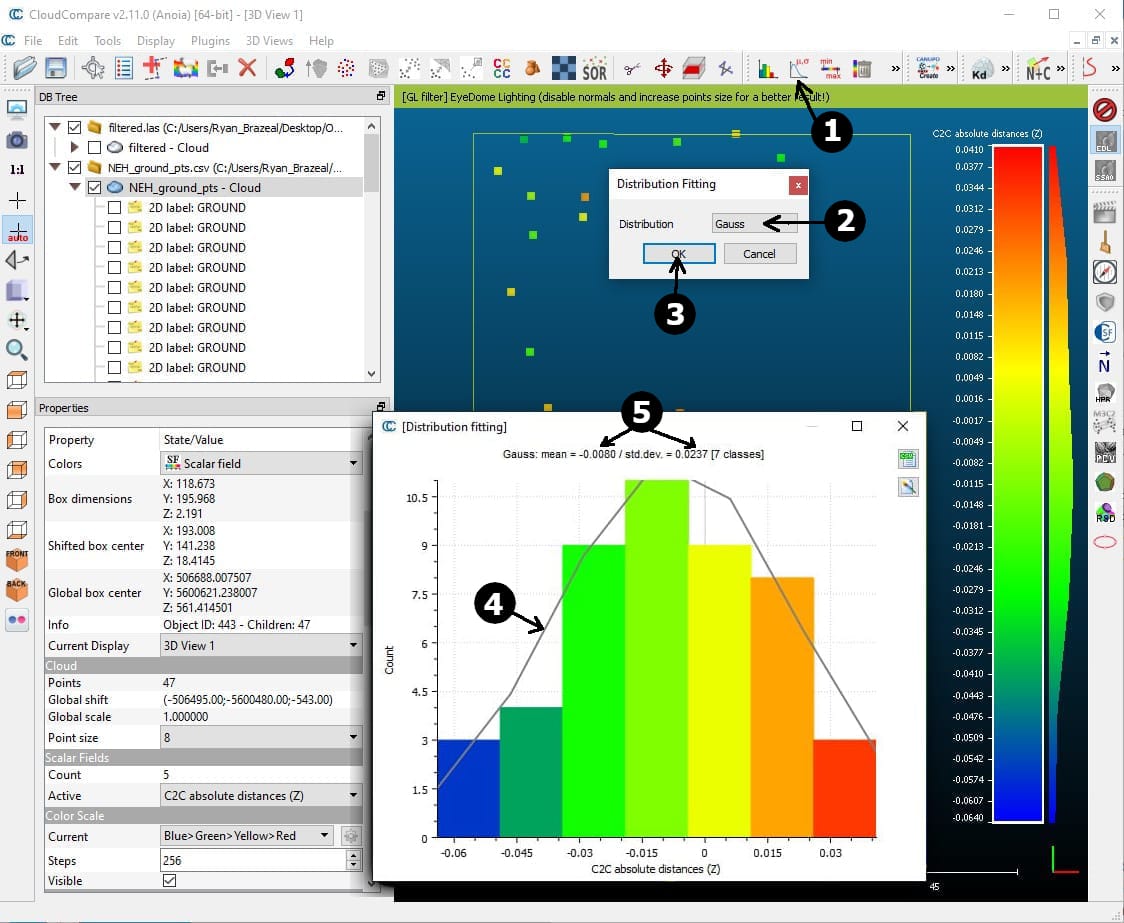
Fig 2.8-3. Ground points colored by height (Z) difference	Fig 2.8-4. Fit Gaussian (normal) distribution to Z differences

---

2.9 Mapping Camera - External Calibration

Attention

The current OpenMMS mapping camera calibration procedure requires using a licensed version of the photogrammetric software, Pix4Dmapper (the free 15-day trial license works perfectly). Future OpenMMS developments also aim to allow the use of Metashape/Photoscan, and OpenDroneMap (ODM) within this camera calibration procedure.

This section presents the last of three calibration procedures that need to be performed on the OpenMMS sensor. The OpenMMS mapping camera calibration procedure can (realistically) only be performed by analyzing MMS data from an RPAS-based data collection campaign. The OpenMMS Sony A6000 Mapping Camera is mounted with its field of view centered around the nadir direction. Therefore, images collected from the sensor while close to the ground will lack the necessary geospatial detail required for the current camera calibration procedure to be effective. The calibration procedure also requires that 3D coordinates (within a realized mapping coordinate system) for a network of pre-surveyed RTK ground control points (GCPs), be known. The ground control points must also be distinguishable within the images collected by the mapping camera.

The final results of this calibration procedure, are the three lever-arm offsets and three boresight angular misalignment angles for the perspective center and optical axis of the mapping camera, with respect to the lidar sensor’s coordinate system. Unlike the lidar sensor’s calibration procedure, these six external calibration parameters need to be re-entered back into the current Applanix POSPac UAV project, and a new exterior orientation (EO) dataset for the collected images needs to be generated and exported. The mapping camera’s external calibration parameters need to be either, re-entered into the settings for every POSPac UAV project, or adjusted within the POSPac UAV project template(s), to be utilized within future OpenMMS projects. In addition to the external calibration parameters, precise estimates for the camera’s interior orientation (IO) parameters are also available from the results of the photogrammetric bundle-block adjustment (BBA) performed by Pix4Dmapper.

Warning

It is well known that the IO estimates for a non-metric camera, generated by a BBA, are usually highly correlated. As a result, the benefit of using the current ‘precise’ IO estimates in future OpenMMS projects may be negligible. That being said, the ‘precise’ IO estimates for a Sony A6000 camera with a Sony 16mm lens are usually not much different than the default IO values. The openmms_preprocess_images.py application (discussed below) also utilizes these default IO values if no other ‘precise’ values are available.

The following discussion outlines how to perform the OpenMMS mapping camera calibration procedure. Start by double checking that the event1_eo… .txt file has been copied from the POSPac UAV Project’s EO subdirectory to the sony_a6000_images subdirectory in the data collection directory, see Figures 2.5-1 and 2.5-2.

7_PREPROCESS_IMAGES

The 7th trigger file, 7_preprocess_images, executes the application openmms_preprocess_images.py. There are NO processing options that can be edited inside this trigger file. Execute this OpenMMS data processing procedure by double-clicking on the 7_preprocess_images file inside the sony_a6000_images subdirectory. This trigger file will be executed a total of three times throughout the OpenMMS data processing. Unlike the other trigger files, the user is prompted to enter the processing options at different times throughout the application’s execution. For the 1st execution of 7_preprocess_images, enter the processing options exactly as shown in the following figure.

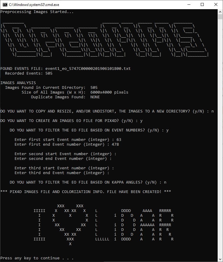
Fig 2.9-1. 7_preprocess_images processing options (1st and 2nd executions)

Warning

It should be noticed that the openmms_preprocess_images.py application determines the number of camera events present within the POSPac generated event1_eo… .txt file, and compares this to the number of .JPG files present within its directory (i.e., the sony_a6000_images directory). These numbers need to match for the processing to continue. The openmms_preprocess_images.py application also analyzes the available metadata for the .JPG files and attempts to determine if any duplicate images are present. If duplicates are detected, the user can instruct the application to move them to a new subdirectory. However, the application cannot (at least currently) detect all the potential issues with the .JPG images and the camera events. Therefore, the user may have to do an additional manual analysis to determine which image corresponds to which camera event. An interested reader should explore POSPac UAV’s Photo ID generation tool, accessible by clicking on the Edit/Create PhotoID File button, as shown in Figure 2.9-6.

Next, create a Pix4Dmapper project and import ALL the Sony A6000 images, the images_pix4d.csv file (generated in the previous step, see Figure 2.9-2), and the NEH_ground_control_pts.csv file found in the demo project’s gnss_reference_data subdirectory. The following video demonstrates how to use Pix4Dmapper to generate the auxiliary files needed to perform the OpenMMS camera calibration. Pay close attention to all the steps as well as the textboxes within the video. Upon completion of the Pix4Dmapper processing, copy the two generated files (i.e., auxiliary files #8 and #9) from the Pix4D project folder -> 1_initial -> params to the sony_a6000_images subdirectory, see Figure 2.9-3.

Attention

For those users who do not have access to Pix4Dmapper software, the two files generated within this section have been included as part of the OpenMMS Demo Project Data, and can be found within the pix4d_exports directory.

Video 4. Pix4Dmapper v4.5.6 demonstration (no audio)

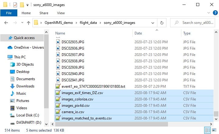
Fig 2.9-2. Results of 7_preprocess_images in subdir.

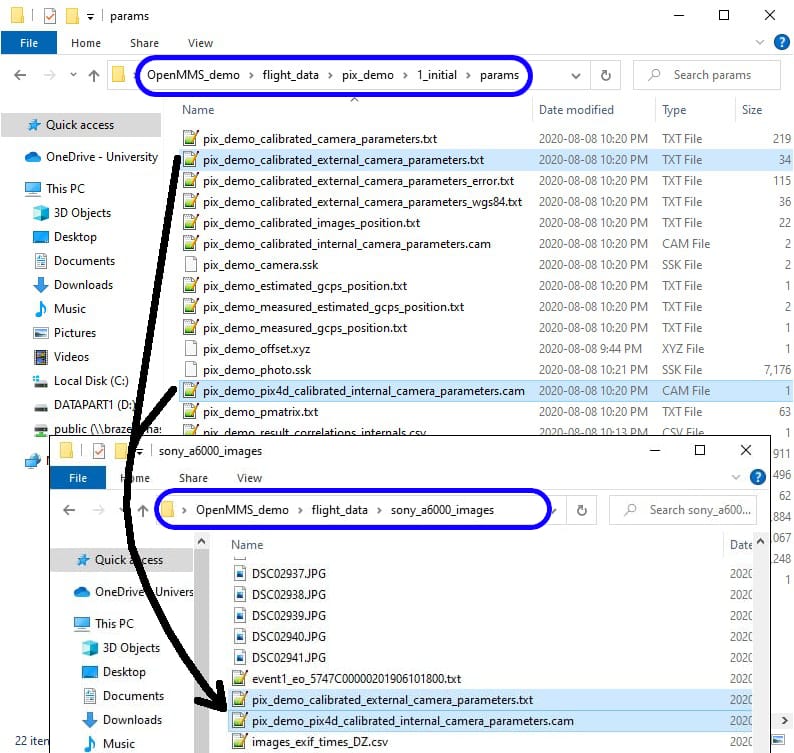
Fig 2.9-3. Pix4D generated files copied to sony_a6000_images subdir.

8_CAMERA_CALIBRATION

The OpenMMS mapping camera external calibration can now be performed. The eighth trigger file, 8_camera_calibration, executes the application openmms_camera_calibration.py and contains two processing option that can be edited. To begin, open the 8_camera_calibration file using a text editor (do not double click on it). The following figure illustrates the one processing option within the trigger file on Windows OS.

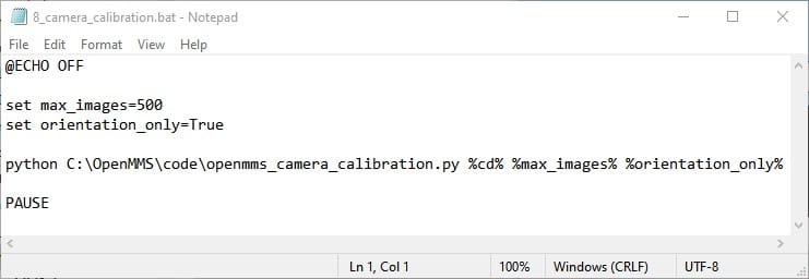
Fig 2.9-4. 8_camera_calibration trigger file contents (Windows)

The two processing options for the openmms_camera_calibration.py application are:

1. max_images: this option specifies the maximum number of images used within the camera calibration mathematical analysis. If max_images is less than the total number of images available, then a subset of the total images is used. The sampling is evenly spaced (as much as possible) from the available images. The default value is 500 images.

2. orientation_only: this option specifies if only the boresight calibration parameters are to be estimated. If orientation_only is set to False, then the lever arm offset values between the origin of the lidar sensor and the perspective center of the camera will also be estimated. The boresight estimates and lever arm estimates are usually very highly correlated. The default value is True.

Execute the 8_camera_calibration trigger file by double-clicking on the file inside the sony_a6000_images subdirectory. The OpenMMS camera calibration procedure performs a least-squares analysis using the observed EO data exported by POSPac UAV, and the control EO data produced by the bundle-block adjustment within Pix4Dmapper. The camera’s external calibration parameters are optimized to minimize the differences between the observed EO data with respect to the control EO data. The results of the camera calibration procedure are displayed directly within the command-line interface dialog (see the blue box in Figure 2.9-5), as well saved to an ASCII-based .log file within the sony_a6000_images subdirectory.

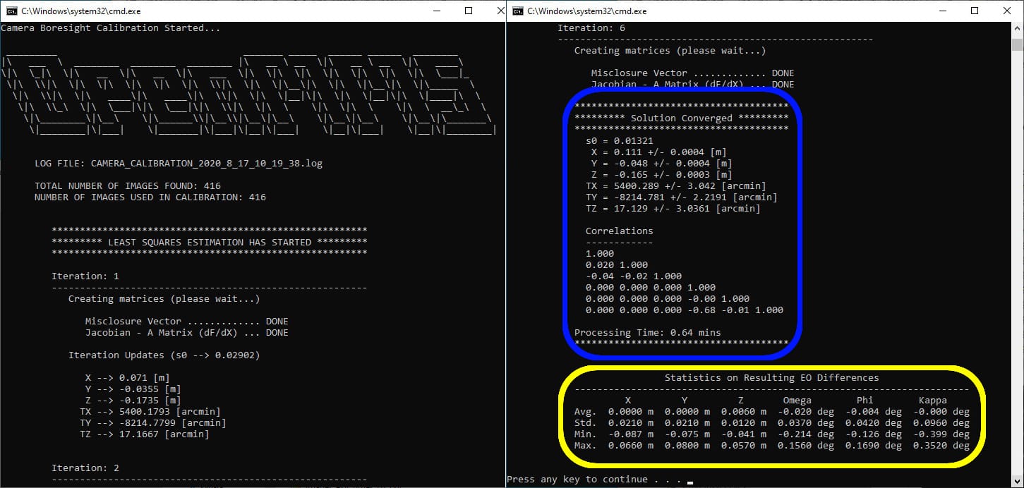
Fig 2.9-5. 8_camera_calibration execution results (saved to .log file)

Next, the camera calibration parameters need to be copied and entered into the POSPac UAV software within the Project Settings -> Camera -> Lever Arms, Boresights and Photo ID -> Reference to Camera Lever Arm and Reference to Camera Boresight Angles sections, see Figure 2.9-6. Re-export the EO dataset for the camera events (which produces the needed auxiliary file #7) by selecting the Tools tab in the POSPac UAV menubar and clicking the Exterior Orientation Processor button, see the 5:38 timestamp in Video 3 for clarification. Next, the re-exported event1_eo… .txt file, found in the POSPav UAV Project’s EO subdirectory, needs to be copied to the sony_a6000_images subdirectory, see Figure 2.9-7.

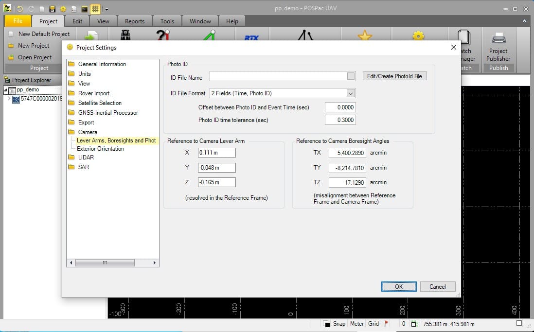
Fig 2.9-6. POSPac Project Settings for camera calibration parameters

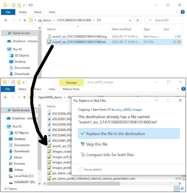
Fig 2.9-7. Update event1_eo… .txt file in sony_a6000_images subdir.

The OpenMMS camera calibration is now complete! However, a few additional processing steps are strongly recommended as a Quality Assurance measure. First, the 7_preprocess_images trigger file needs to be executed for the 2nd time. Enter the processing options exactly as shown in Figure 2.9-1. This processing will produce a new images_pix4d.csv in the sony_a6000_images subdirectory.

Reopen the Pix4Dmapper project, and open the Image Properties Editor dialog, see Figure 2.9-8. Click the Clear button to remove the previous EO parameters (i.e., X, Y, Z, Omega, Phi, Kappa). Click the From File… button. Within the Select Geolocation File dialog that appears, select the X,Y,Z File Format. Browse to the new images_pix4d.csv file and select it. Close the open dialogs by clicking either the Open or OK button.

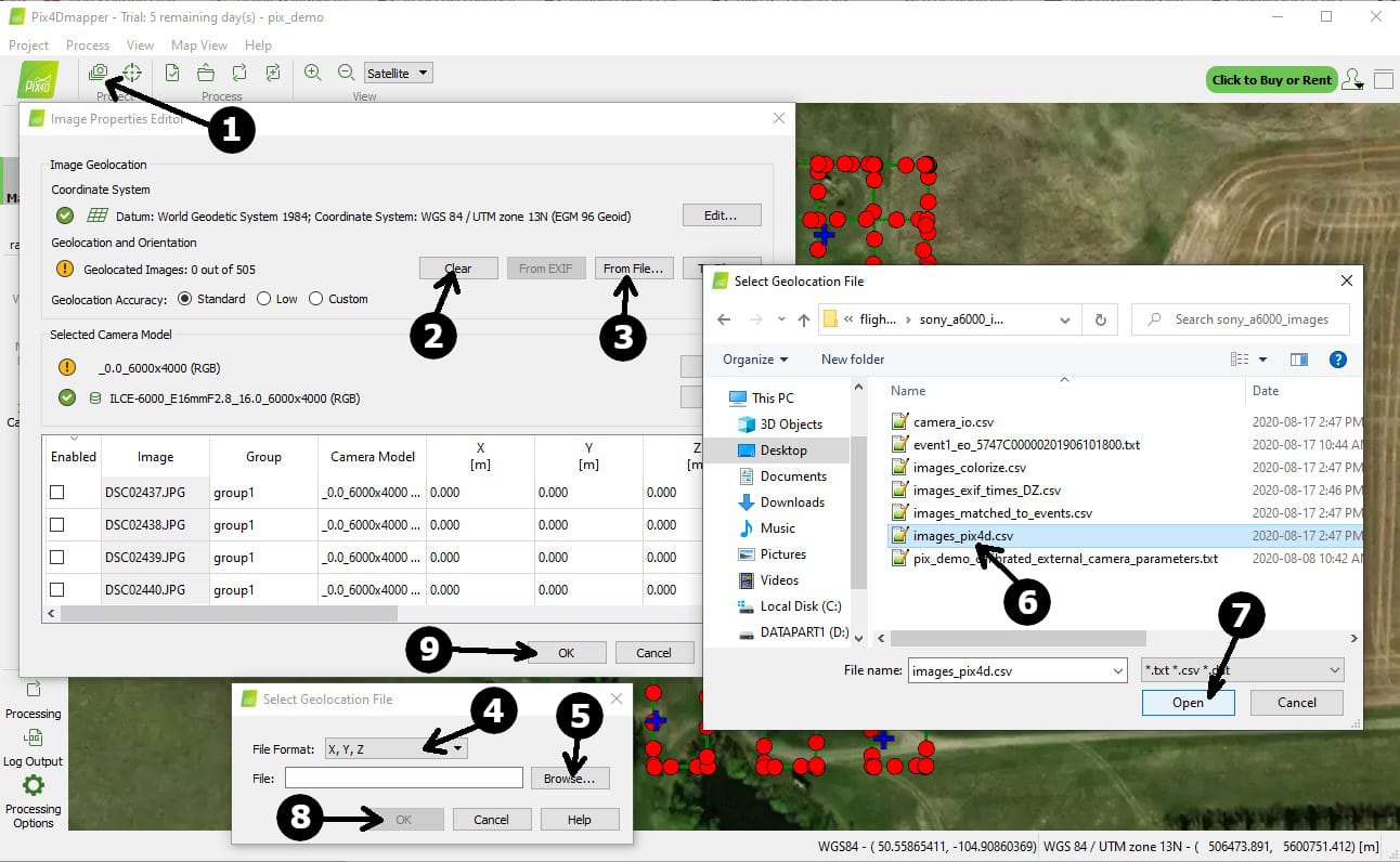
Fig 2.9-8. Pix4Dmapper Image Properties Editor dialog

Open the GCP/MTP Manager dialog, see Figure 2.9-9. Click anywhere within the first row of the table to select the GCP. While holding the SHIFT key, click anywhere within the last row of the table to select ALL the GCPs. Right-click anywhere within the Type column and select Edit Types in Selected Rows. Change all the GCPs to the Check Point type. Click OK to save and close the dialog.

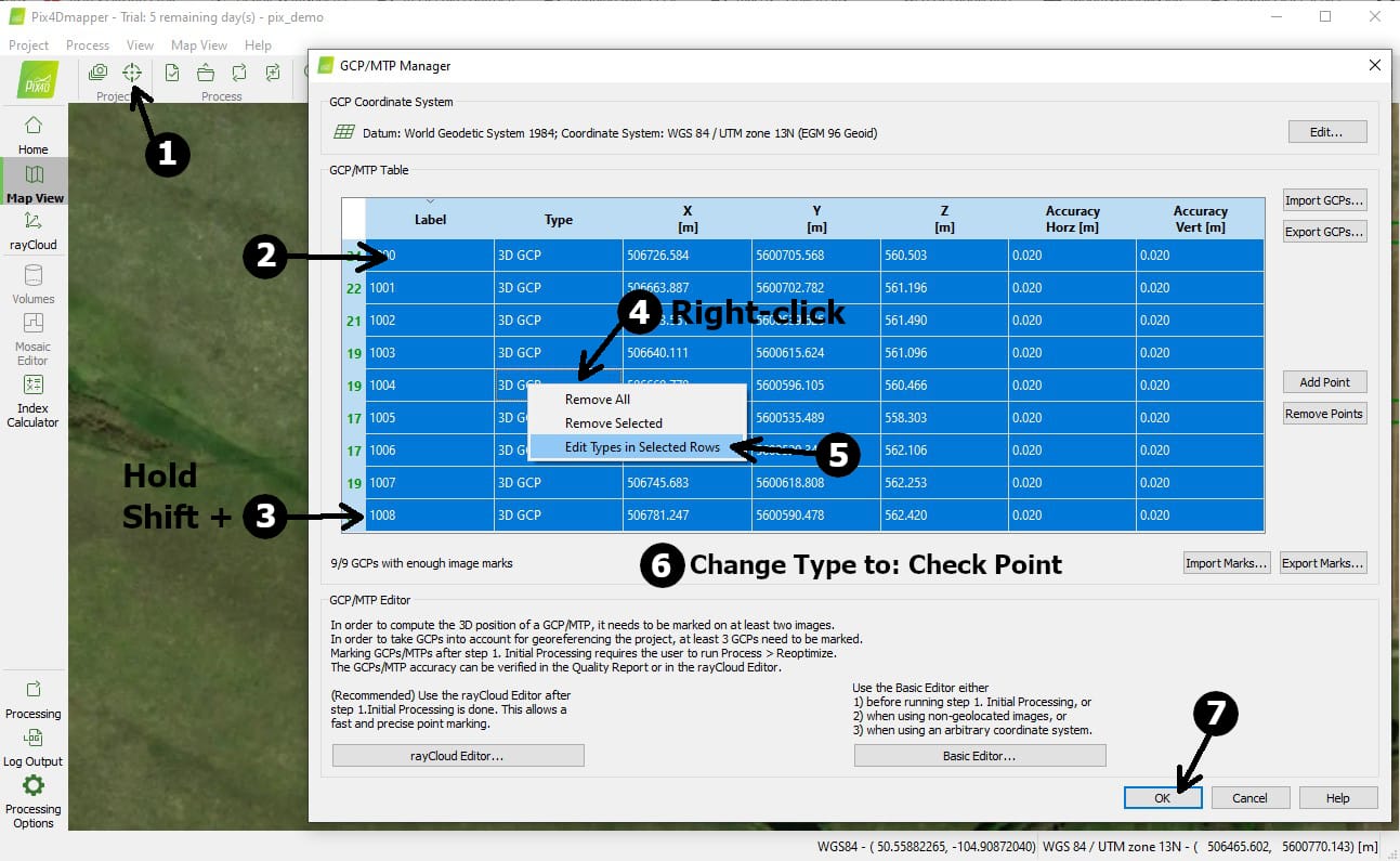
Fig 2.9-9. Pix4Dmapper GCP/MTP Manager dialog

Click the Processing Options button in the bottom-left corner of the Pix4Dmapper application. On the Processing Options dialog that appears (see Figure 2.9-10), select the 1. Initial Processing item from the list, and select the Calibration tab. Change the Calibration Method from Standard to Accurate Geolocation and Orientation. Before clicking the OK button, make sure that ONLY the 1. Initial Processing item is checked, and the other two items are NOT checked.

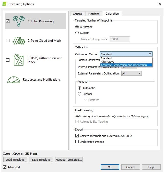
Fig 2.9-10. Pix4Dmapper Processing Options dialog

Once the edits to the images’ EO parameters, the GCPs’ types, and the processing options have been made, the Pix4Dmapper project needs to be Reoptimized. From the main menu at the top of the Pix4Dmapper application, select the Process menu, and click on Reoptimize. It is ok to overwrite the previous processing results when prompted. Once the progress bar near the bottom-left corner of the application reports Done, Regenerate Quality Report from the menu, if needed., the final step is to click on Generate Quality Report from the Process Menu. Once the Quality Report has been generated, it will be automatically displayed on the screen.

Examine the Geolocation Details section near the end of the report. Within the Ground Control Points section, the Mean [m] values for the Errors in X, Y, Z should all be nearly zero, and the Sigma [m]/RMS Error [m] values should all be 2-5cm (ideally), see Figure 2.9-11. This analysis represents the positional error witnessed on the ground at the locations of the GCPs. Within the Absolute Geolocation Variance section, a tabular error distribution for the Errors in the X, Y, Z coordinates of the images is presented, see Figure 2.9-12. Ideally, these distributions should closely conform to a Gaussian distribution. This analysis represents the positional error witnessed at the camera locations, and not on the ground. Lastly, the Geolocation Orientational Variance table discusses the Euler rotation angles (e.g., Omega, Phi, Kappa) that define the direction of the camera’s optical axis when each image was taken. The RMS [degree] values for each angle, based on the differences between the initial POSPac EO data and the BBA EO data, are presented. Ideally, these values should be very close to the boresight estimates from the camera calibration procedure (examine the values in the yellow box in Figure 2.9-5).

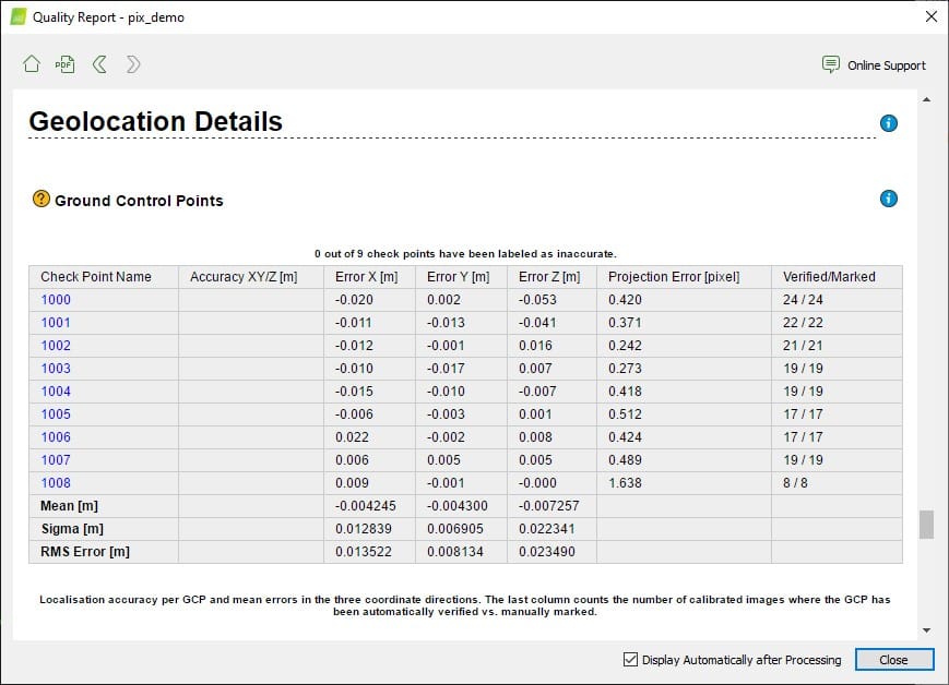
Fig 2.9-11. Geolocation Details - GCPs

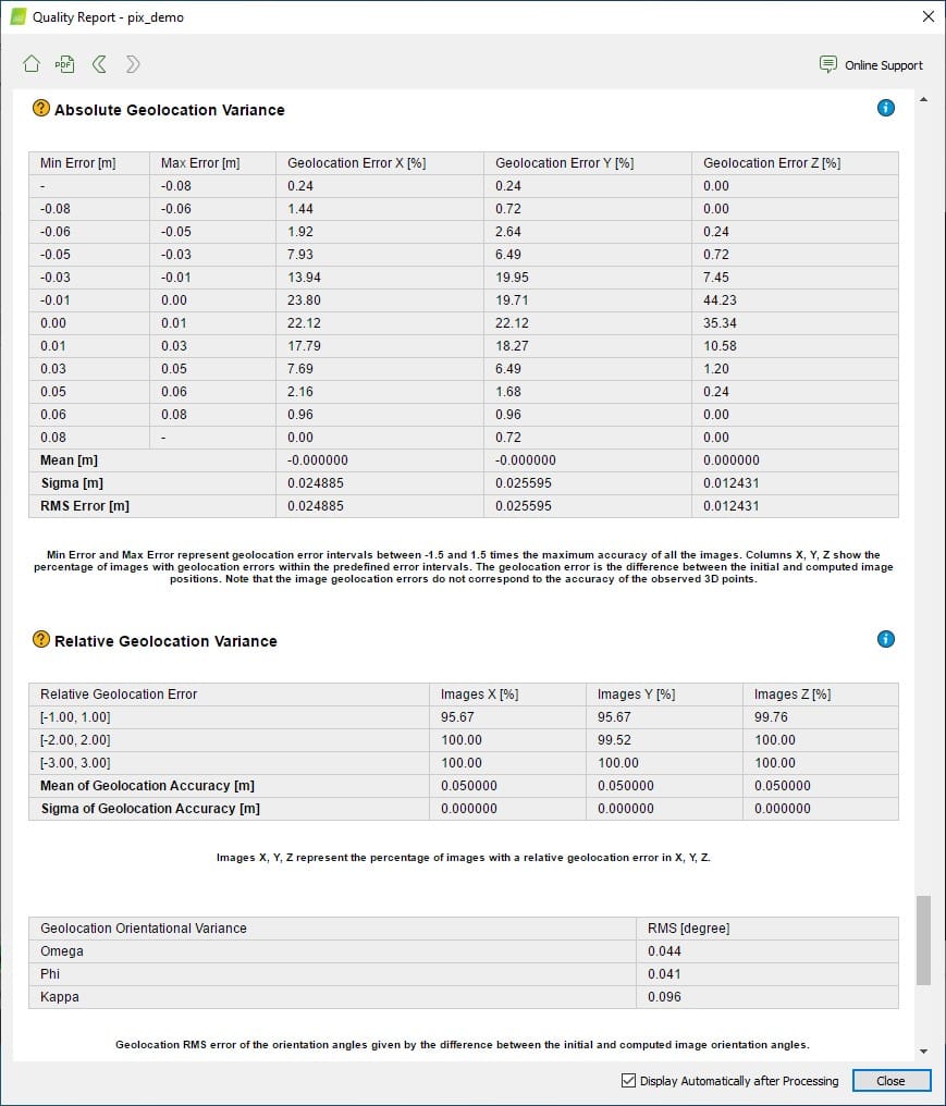
Fig 2.9-12. Geolocation Details - Position and Orientation Differences

---

2.10 Point Cloud Colorization

It was essential to develop and include a rigorous point cloud colorization solution within the currently offered OpenMMS suite of open-source software applications. The OpenMMS point cloud colorization procedure offers several processing options. The options allow for the real-world color of a lidar observed point to be determined using:

1. The mapping camera image that was taken at the time epoch closest to when the point was observed.

2. The mapping camera image that was taken at the position closest to the observed point.

3. A balanced (i.e., blended) color computed using up to three of the closest mapping camera images (based on time or position).

The OpenMMS point cloud colorization procedure utilizes the perspective geometric relationship between the lidar observed points and the mapping camera images to determine which image pixel corresponds to each lidar observed point. Therefore, an orthorectified mosaic is not utilized within the OpenMMS point cloud colorization procedure. Using perspective imagery within the colorization procedure allows for features that would be occluded within orthorectified imagery to be colorized more rigorously.

Begin the OpenMMS point cloud colorization procedure by executing the 7_preprocess_images trigger file for the 3rd (and final) time. Enter the onscreen processing options exactly as shown in Figure 2.10-1.

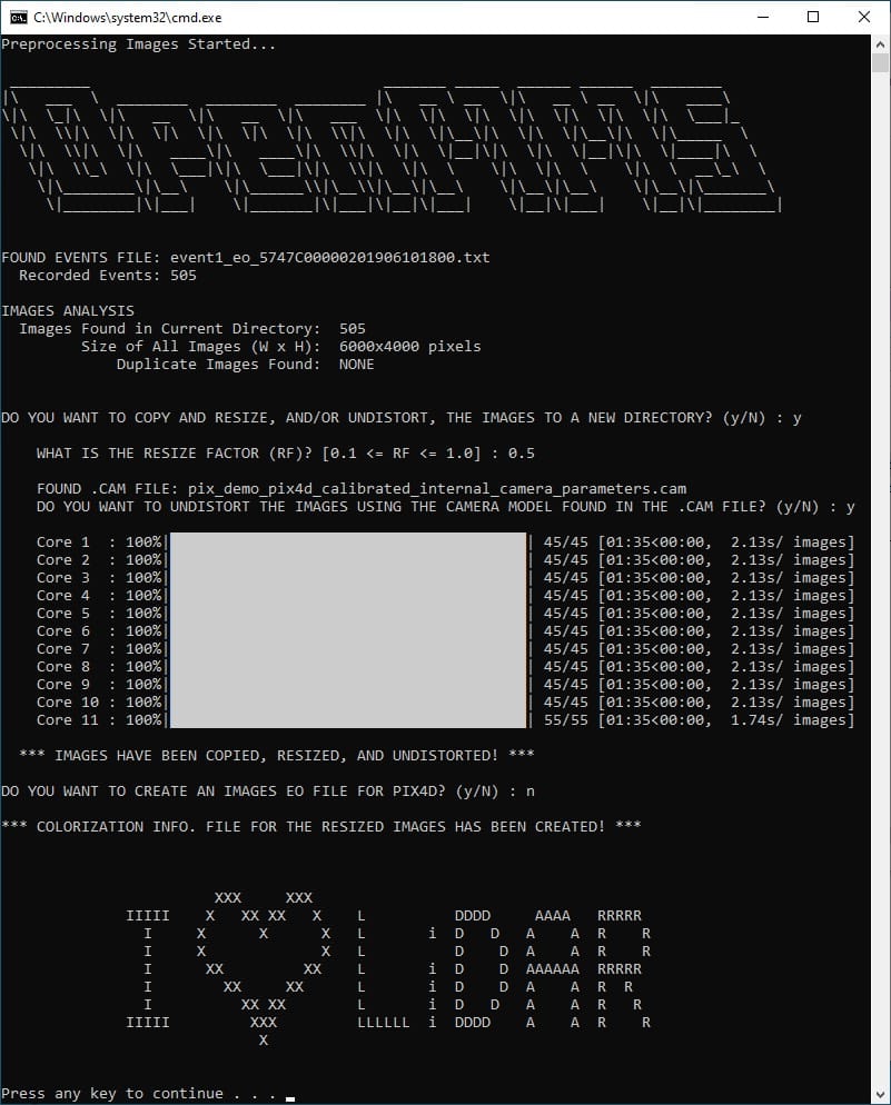
Fig 2.10-1. 7_preprocess_images processing options (3rd execution)

The result of this processing step is the creation of a new subdirectory within the sony_a6000_images directory, named resized_X.Y, see Figure 2.10-2. Within the resized_X.Y subdirectory, copies of all of the original mapping camera images resized by the factor * X.Y* are generated. Additionally, the user can select if the original images should also be undistorted based on either, the ‘precise’ IO parameters estimated within the Pix4D processing (made available via the .cam file), or the default set of IO parameters for a Sony A6000 camera (with 16mm lens). Lastly, the 9_colorize_las trigger file needs to be moved from inside the sony_a6000_images directory, and put inside the new resized_X.Y subdirectory, see Figure 2.10-3.

Tip

It is strongly recommended to resize the original images by a minimum value of 0.5 and undistort the images based on either a .cam file or the default values. By resizing and undistorting the images the colorization procedure will be more computer memory friendly, faster, and the colorization results will still be excellent!

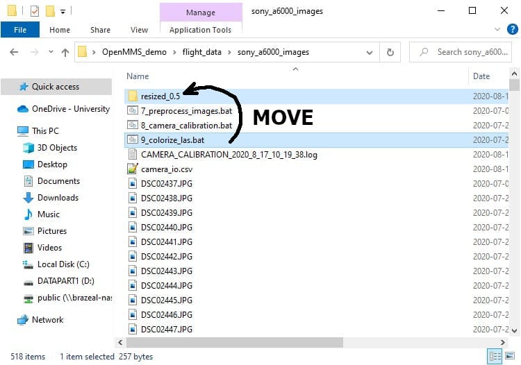
Fig 2.10-2. New resized_X.Y subdirectory

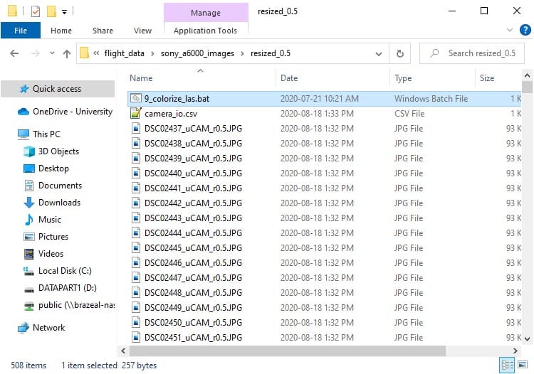
Fig 2.10-3. Contents of the new resized_X.Y subdirectory

9_COLORIZE_LAS

The OpenMMS point cloud colorization procedure can now be performed. The ninth trigger file, 9_colorize_las, executes the application openmms_colorize.py and contains three processing options that can be edited. To begin, open the 9_colorize_las file using a text editor (do not double click on it). The following figure illustrates the three processing options within the trigger file on Windows OS.

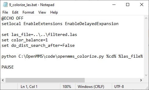
Fig 2.10-4. 9_colorize_las trigger file contents (Windows)

The three processing options for the openmms_colorize.py application are:

1. las_file: this option specifies the relative path, from the current directory, and filename for the .las point cloud file to be colorized. The default value is ..\ ..\filtered.las (Windows) or ../../filtered.las (Mac/Linux) which indicates that the .las file to be colorized is named filtered.las and it exists within the grandparent directory (i.e., up 2 hierarchy levels from the current directory).

Warning

Windows OS uses \ characters within path strings, while Mac OS and Linux distros use / characters. Be careful to use the correct syntax.

2. color_balance: this option specifies the number of closest images (time-based or distance-based) to be used to compute the balanced color for each observed point. The default value is 1 (valid options are 1-3 inclusive).

3. do_dist_search_after: this option specifies if a secondary distance-based colorization procedure should be performed after the primary time-based colorization procedure has completed. Only the remaining uncolored points will be analyzed within the secondary colorization procedure. The default value is False.

Execute the 9_colorize_las trigger file by double-clicking on the file inside the resized_X.Y subdirectory. The result of the point cloud colorization procedure is a new colorized .las point cloud file generated within the same directory as the specified las_file processing option. IMPORTANT NOTE: it is possible that the new colorized point cloud dataset will be saved as multiple .las files. This attempts to fix an odd 32 bit issue that was experienced during development. A notice message near the top of the command-line dialog for the point cloud colorization procedure will alert the user if multiple .las files will be created, see Figure 2.10-5.

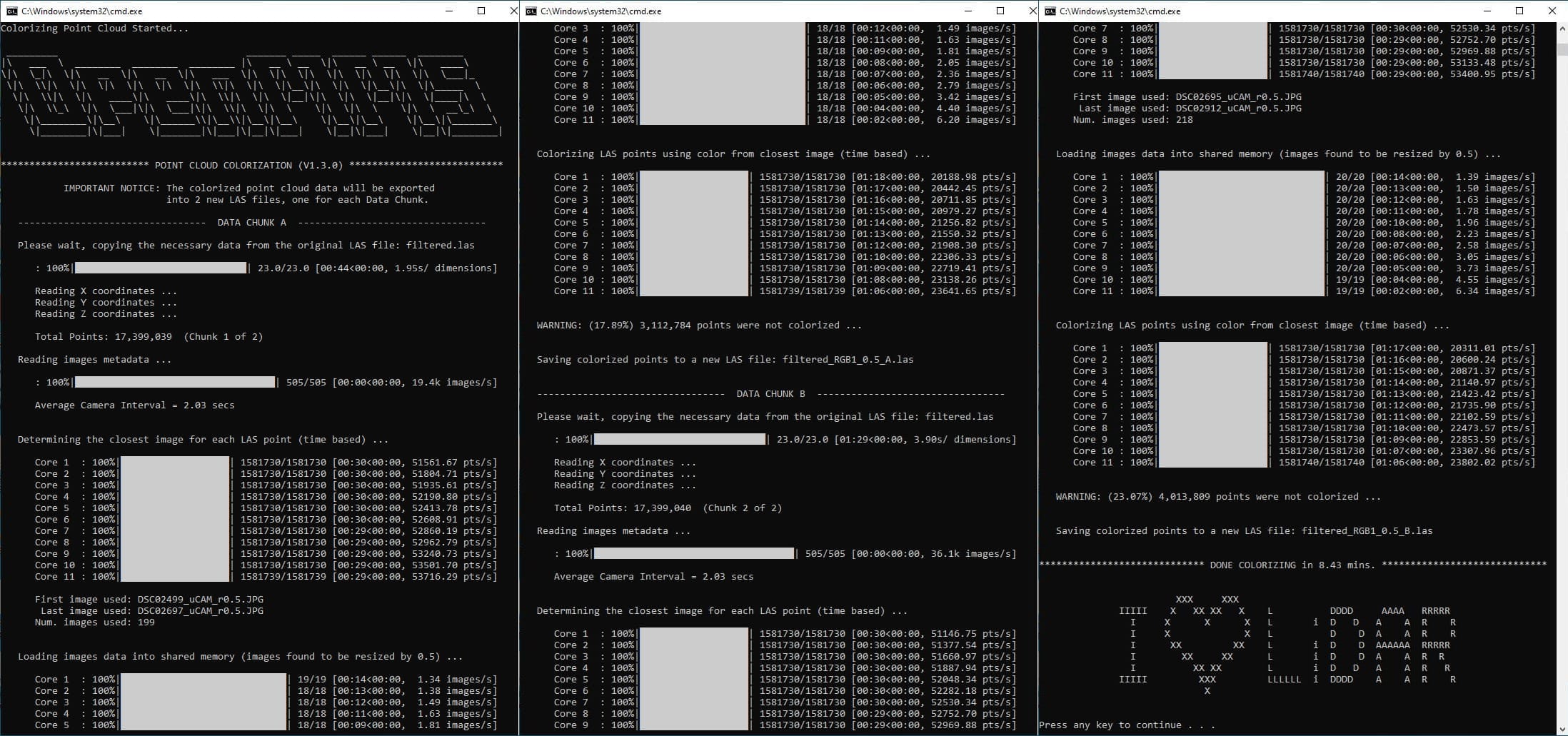
Fig 2.10-5. 9_colorize_las execution results (using default processing options)

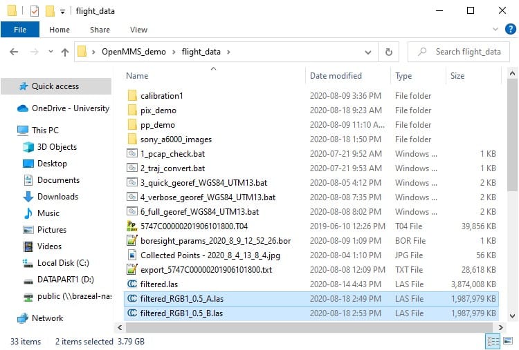
Fig 2.10-6. New colorized .las point cloud file(s)

The new file(s) can be opened within CloudCompare to view the colorized point cloud and merge the multiple point clouds into a single .las (or other) point cloud file format, if desired. An OpenMMS colorized point cloud contains two additional point attributes (i.e., scalar fields in CloudCompare). The two attributes are:

1. image_used: this specifies the index number of the image used to colorize the point. The index numbers start at 1 for the first mapping camera image. A value of 0 indicates that no mapping camera image was found that contained the point. By filtering based on this attribute, the user can isolate a subset of the point cloud that covers the field of view of a specific mapping camera image for further investigation or research purposes.

2. color_class: this specifies the color class number for the point. A value of 0 indicates that the point has not been colorized. A value of 1 indicates that the point was colorized using the closest time-based image(s). Lastly, a value of 2 indicates that the point was colorized using the closest distance-based images(s). By filtering based on this attribute, the user can isolate only the colorized (or uncolorized) points within the entire point cloud, see the figures below.

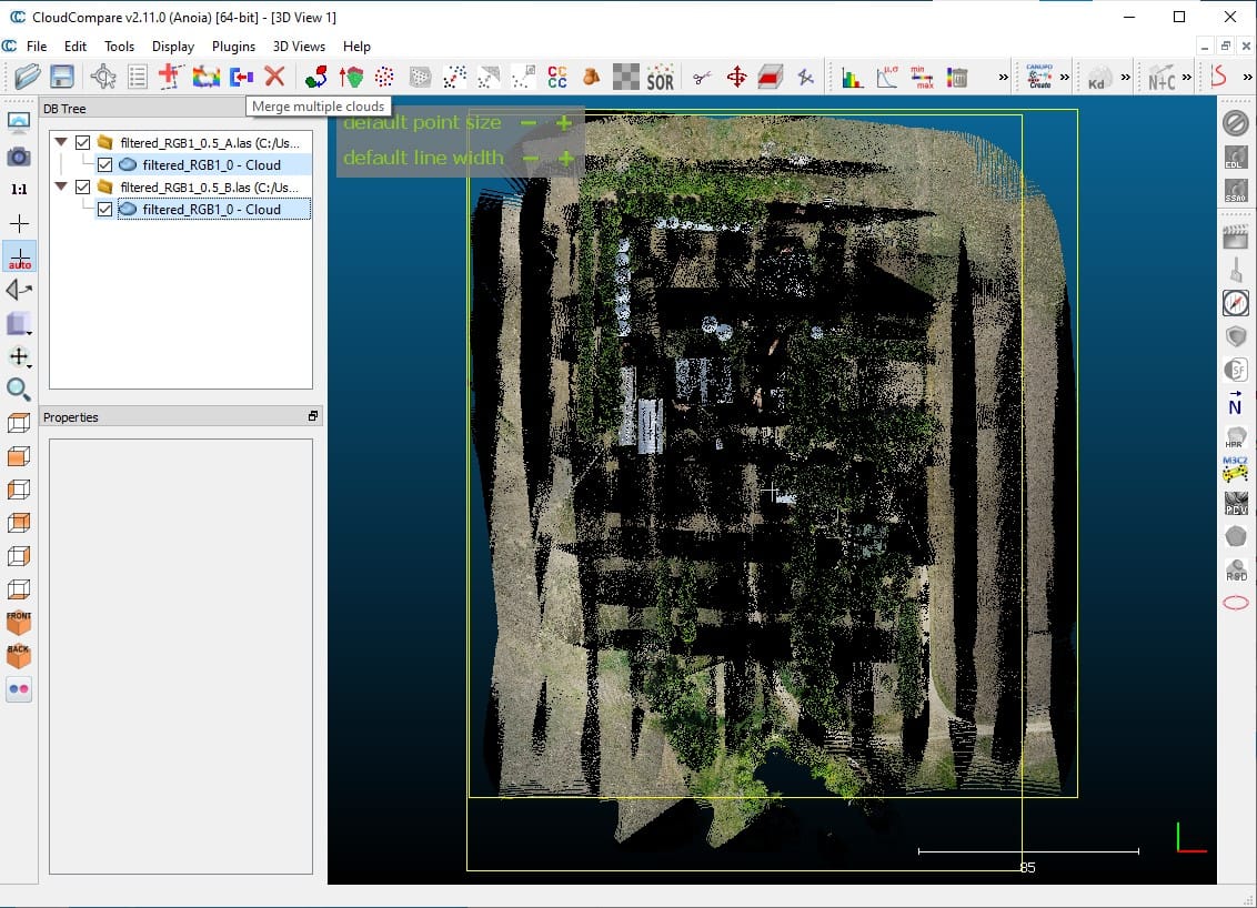
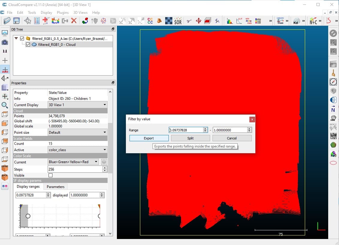
Fig 2.10-7. Colorized point clouds with mixed color classes	Fig 2.10-8. Filtering the color class to values > 0 (i.e., colored pts.)
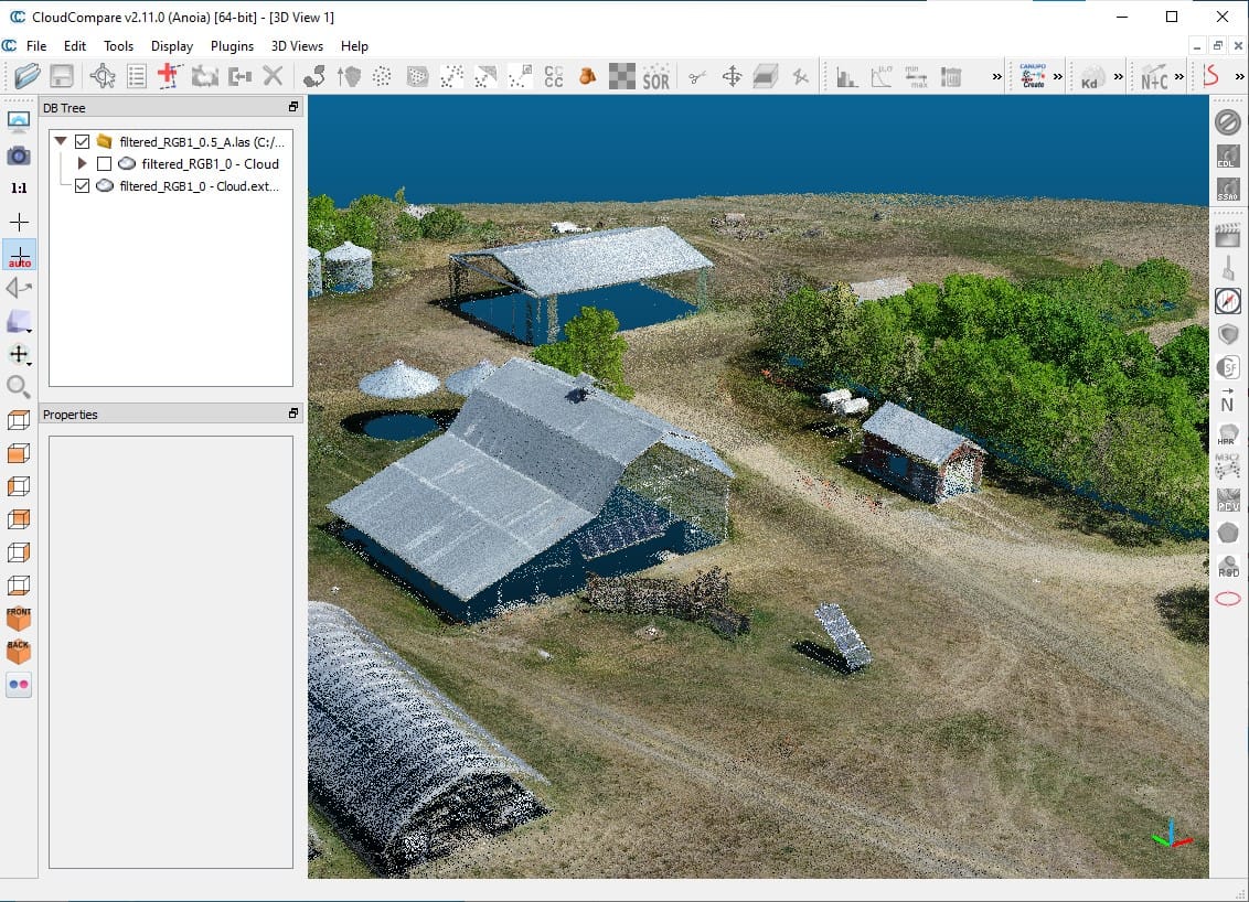
Fig 2.10-9. Colorized point cloud with only colorized points	Fig 2.10-10. Perspective view of the colorized point cloud

---

3. Data Processing Tutorial #2

Attention

The demo project’s lidar data was collected using an OpenMMS sensor with a Livox MID-40 lidar scanner. Therefore, the following documentation discusses and showcases the OpenMMS data processing workflow for sensors with a Livox MID-40.

See Data Processing Tutorial #1 (above) if you are interested in the OpenMMS data processing workflow using Velodyne VLP-16 lidar data.

3.1 Demo Project Data (MID-40)

OpenMMS Open Data License

Copyright Ryan G. Brazeal 2020.

This OpenMMS Demo Project Data (MID-40) is made available under the Open Database License: https://opendatacommons.org/licenses/odbl/1.0/. Any rights in individual contents of the data are licensed under the Database Contents License: https://opendatacommons.org/licenses/dbcl/1.0/.

Click Here to Download the OpenMMS Demo Project Data (MID-40), approx. 3 GB .zip archive

The Demo Project Data (MID-40) is for an RPAS-Lidar mapping project collected with an OpenMMS v1.3 sensor. The data was collected on October 1st, 2020, over a rural property near Saskatoon, Saskatchewan, Canada. The OpenMMS sensor was flown on a Freefly Alta X RPAS at an altitude of ~ 67 m above ground level (AGL), at a horizontal speed of ~ 5 m/s, mapping images were taken every ~ 2 sec, and a video of the flight was recorded. The included OpenMMS datasets are:

1. GNSS-INS observations from an Applanix APX-18 sensor, .T04 file

2. Lidar observations from a Livox MID-40 sensor, .pcap file

3. Real-time trajectory observations from an Applanix APX-18 sensor, .traj file (ASCII)

4. Nadir view video from the RPAS, .mp4 file (unfortunately the lens was slightly out of focus)

5. Nadir view images from a Sony A6000 camera, .JPG files (313 in total)

6. Time synchronization reference, .livox file (ASCII)

The included auxiliary datasets are:

1. GNSS observations from a Trimble R10 reference station, .T02 file

2. Geodetic coordinates and datum information for the reference station, .txt file

3. RTK surveyed ground control points/targets positioned across the project site, .csv file

4. RTK surveyed points on the terrain/ground across the project site, .csv file

5. Post-processed trajectory data for the lidar sensor, .txt file

6. Post-processed trajectory data for the Sony A6000 camera, .txt file (before camera calibration)

7. Post-processed trajectory data for the Sony A6000 camera, .txt file (after camera calibration)

8. Bundle adjusted exterior orientation parameters for each image, .txt file

9. Bundle adjusted interior orientation parameters for the Sony A6000 camera, .cam file (ASCII)

NOTE: The auxiliary datasets #5 to #9 will be created as part of the data processing workflow. These files are generated by 3rd party commercial software (either Applanix POSPac UAV or Pix4Dmapper) and are included within the Demo Project to allow interested users, who don’t have access to POSPac UAV or Pix4Dmapper, to still follow along and successfully process the data.

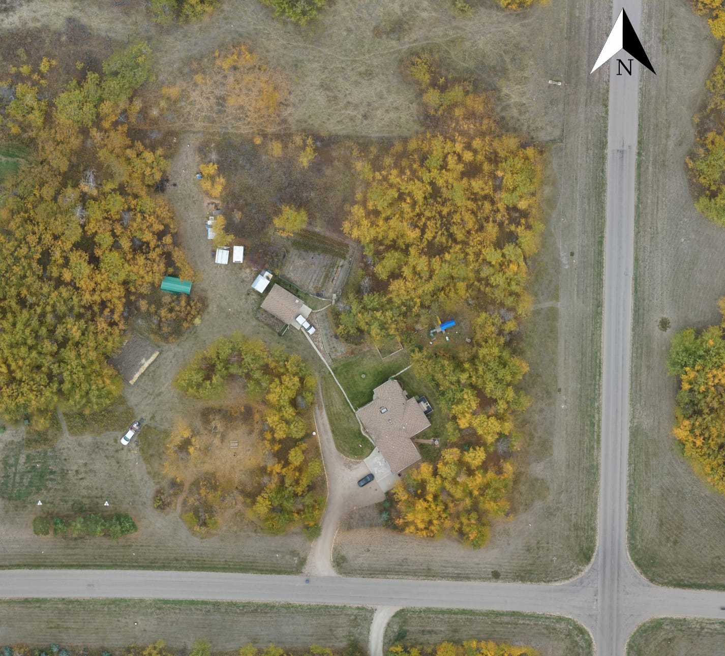
Fig 3.1-1. Demo 2 project area of interest

Attention

The instructions within the following sections were documented using a computer with 32 GB of memory, a NVidia graphics card, and running Windows 10. The tutorial has also been completed (minus the POSPac UAV and Pix4Dmapper processing steps) on a MacBook Pro computer with 16 GB of memory and running Mac OS Mojave. To date, no computers running a Linux OS distro have been tested, though they should work with little to no modifications to the tutorial.

---

3.2 Data Management

It is required to store the files collected by an OpenMMS sensor within an empty directory for each data collection campaign. The OpenMMS sensor firmware automatically increments the names of the collected files for each successive data collection campaign. The names of the collected files make it easy to understand which files relate to the individual data collection campaigns.

Open the directory containing the extracted OpenMMS demo project data. The following figure illustrates the contents of this directory.

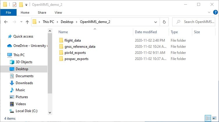
Fig 3.2-1. OpenMMS project directory

Inside the flight_data directory, the six OpenMMS datasets, as described in the previous section, are included and represent the data collected within a single data collection campaign (i.e., a single RPAS flight in the case of the Demo Project). The images obtained from the Sony A6000 mapping camera are included within the directory, sony_a6000_images. To decrease the size of the Demo Project Data by approximately 306 MB, a total of 36 images were replaced with solid black images. The need for the images to be replaced with solid black images, rather than just deleting them, will be explained in an upcoming section.

Warning

It is strongly recommended to use the underscore character instead of the space character when naming a directory or file that contains OpenMMS data.

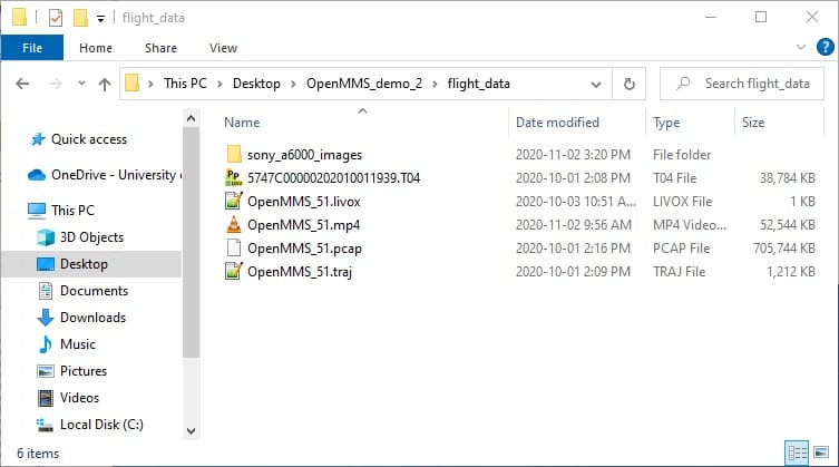
Fig 3.2-2. OpenMMS data collection directory

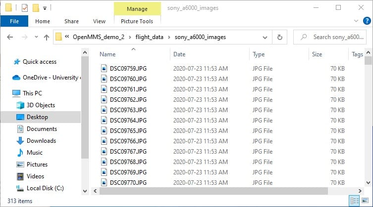
Fig 3.2-3. Sony A6000 images directory

---

3.3 Setup Trigger Files

Attention

The demo project’s lidar data was collected using an OpenMMS sensor with a Livox MID-40 lidar scanner. Therefore, the following documentation discusses and showcases the OpenMMS data processing workflow for sensors with a Livox MID-40.

Be sure to copy the trigger files 1, 3, 4, 5, and 6 that include _livox within their names.

Important

The OpenMMS processing options available within each trigger file will be discussed in full detail within the upcoming section, where the respective trigger file is first used. Full details are not included here.

The next step is to COPY the respective trigger files from the OpenMMS software installation location to the data collection directory. Once inside the data collection directory, the trigger files 7, 8, and 9 need to be MOVED to the sony_a6000_images directory.

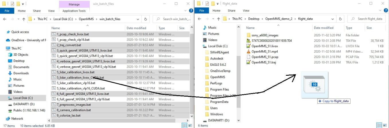
Fig 3.3-1. ALL Windows OS trigger files (.bat) being copied

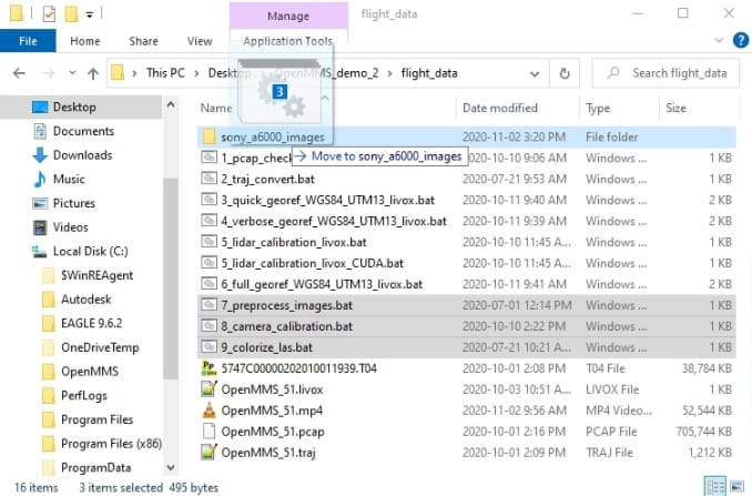
Fig 3.3-2. Mapping camera trigger files being moved

---

3.4 In the Field - Data Processing & QA

The OpenMMS trigger files 1, 2, and 3 are ideally utilized while still in the field immediately after a data collection campaign has finished. The primary goal is to analyze the collected mapping data to ensure that certain characteristics for the point cloud dataset have been achieved (i.e., coverage area, redundancy/overlap, continuous data, etc.).

1_PCAP_CHECK

The 1st trigger file, 1_pcap_check_livox, executes the application openmms_pcap_check_livox.py. There are NO processing options that can be edited inside this trigger file. Execute the first OpenMMS data processing procedure by double-clicking on the 1_pcap_check_livox file inside the data collection directory. Before execution begins, the 1_pcap_check_livox trigger file searches its directory for files with the .pcap file extension and the .livox file extension. Only a single .pcap file and a single .livox file can be present within the directory for execution to start. Error messages will be reported if no .pcap file or no .livox file exists or if multiple .pcap files or .livox files exist.

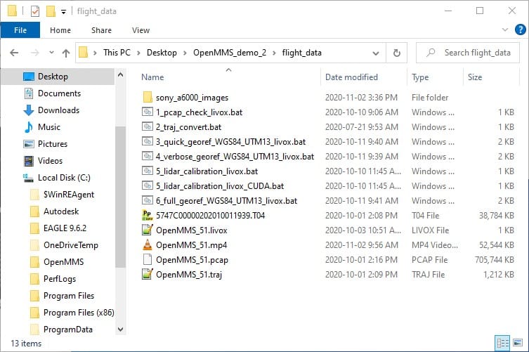
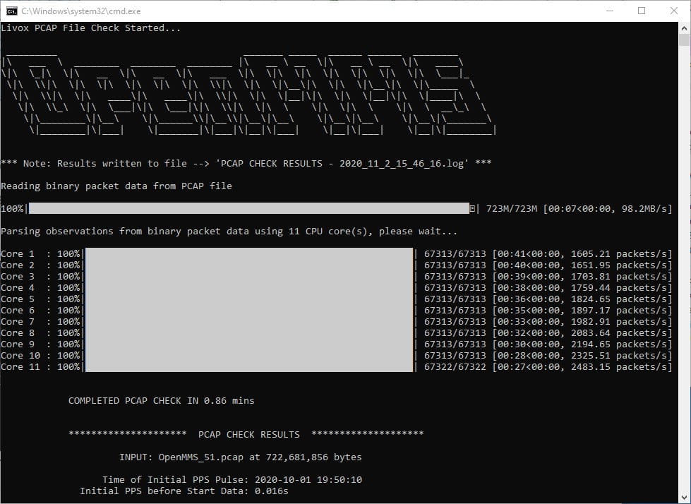
Fig 3.4-1. Directory before executing 1_pcap_check_livox	Fig 3.4-2. 1_pcap_check_livox multi-core processing (saved to file)
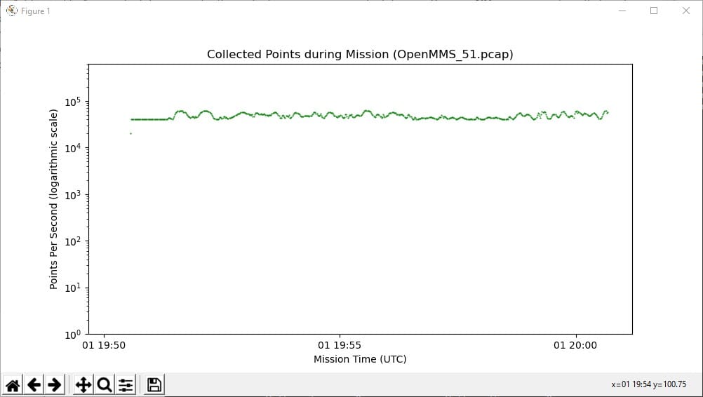
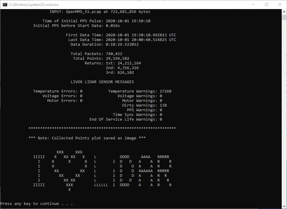
Fig 3.4-4. Collected lidar points during campaign (saved to file)	Fig 3.4-5. 1_pcap_check_livox analysis results (saved to file)

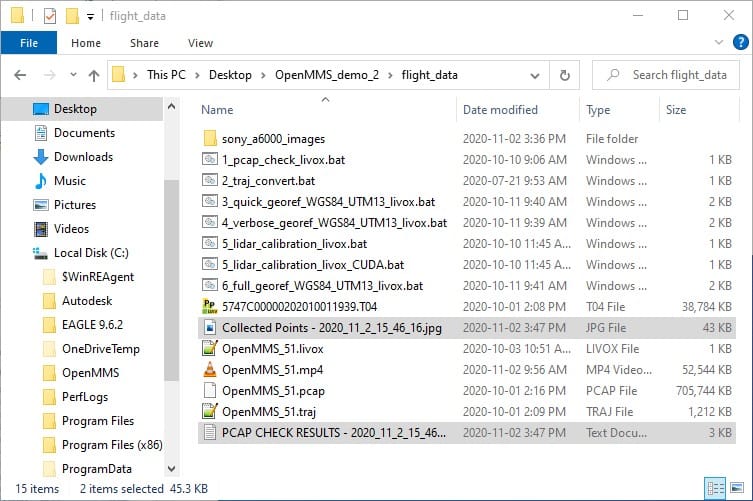
Fig 3.4-6. Directory after executing 1_pcap_check_livox

1_pcap_check_livox generates two useful quality assurance deliverables about the collected lidar data. Figure 3.4-4 illustrates the number of valid lidar points (i.e., where the distance observation was not zero) collected for each second of the data collection campaign. Any times when little or no lidar points were being collected will be visible within this plot. Analyzing this plot can lead to improved confidence that adequate and desirable lidar data was collected. Figure 3.4-5 illustrates the valuable quality assurance metadata about the collected lidar data extracted using 1_pcap_check_livox. These two deliverables are saved to individual files (1 .jpg and 1 ASCII .log) within the data collection directory, as shown in Figure 3.4-6.

2_TRAJ_CONVERT

The 2nd trigger file, 2_traj_convert, executes the application openmms_traj_convert.py. There are NO processing options that can be edited inside this trigger file. Execute the second OpenMMS data processing procedure by double-clicking on the 2_traj_convert file inside the data collection directory. Before execution begins, the 2_traj_convert trigger file searches its directory for files with the .traj file extension. Only a single .traj file can be present within the directory for execution to start. Error messages will be reported if no .traj file exists or if multiple .traj files exist.

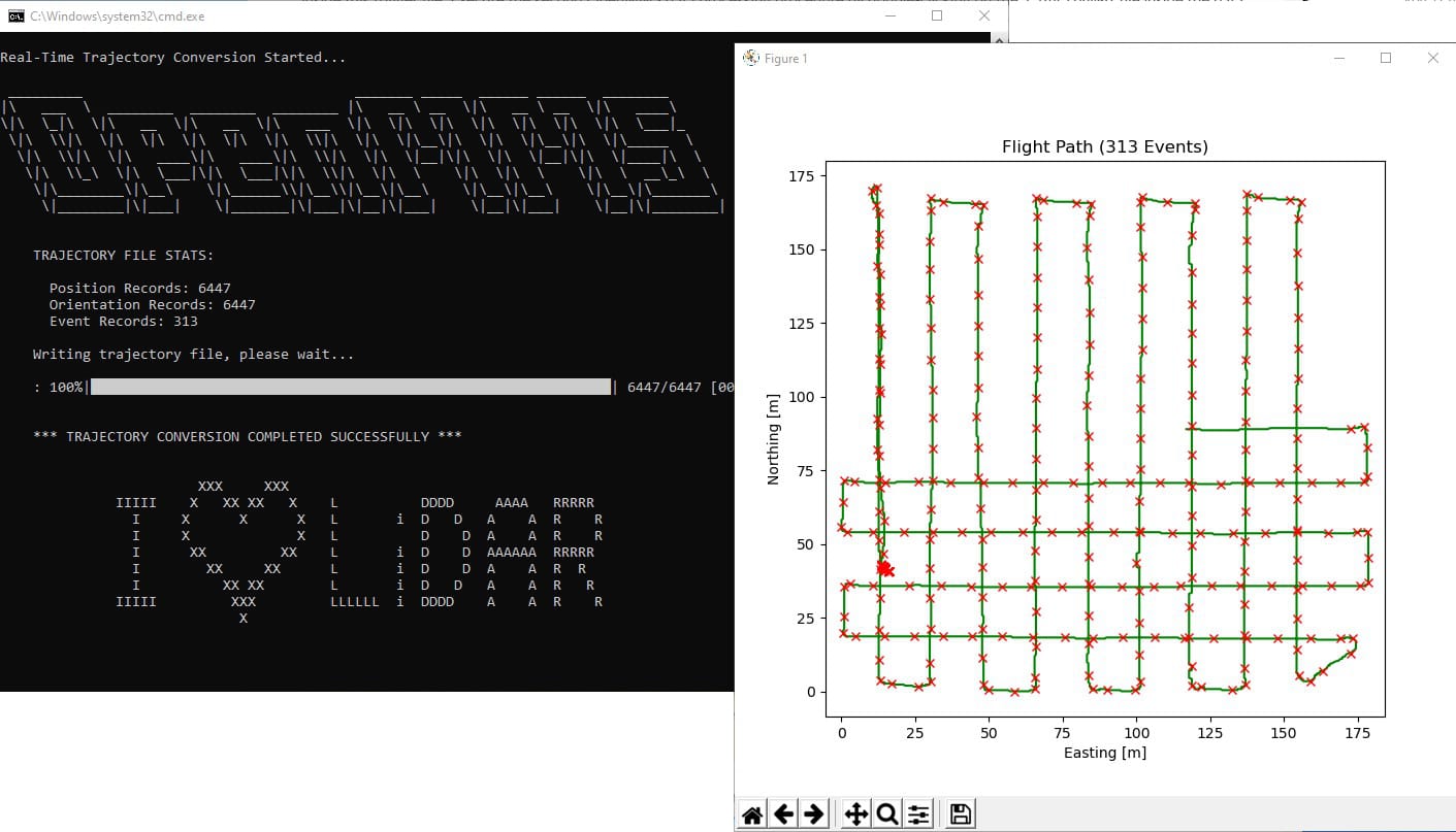
Fig 3.4-7. 2_traj_convert processing and trajectory plot

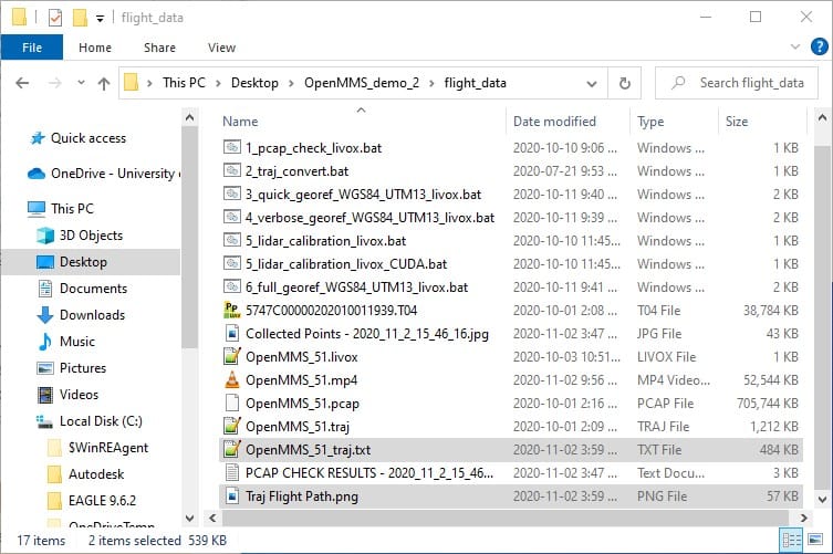
Fig 3.4-8. Directory after executing 2_traj_convert

2_traj_convert generates one useful quality assurance deliverable about the collected Sony A6000 images. Figure 3.4-7 illustrates the plan view plot/map of the lidar sensor during the data collection campaign. This plot places X markers at positions where a Sony A6000 camera image was collected. The total number of camera events (i.e., collected images) is listed in the plot’s title and also displayed within the processing results. This plot is saved to a .png file within the data collection directory, as shown in Figure 3.4-8.

Warning

The total number of camera events reported within this step, may be incorrect. Commonly, 1-2 fewer images are reported. Fewer images are reported when the data collection is stopped just before an image was to be taken. Do not be alarmed if the reported total number of camera events does not precisely match the number of images collected by the Sony A6000 camera. It should be within 1 or 2 images.

Lastly, as the name of the 2_traj_convert trigger file implies, the main purpose of this processing step is to convert the raw, real-time trajectory information (i.e., times, positions, and orientations) for the lidar sensor, into a defined format, ASCII-based .txt file. This .txt file is used within the next processing step and provides the capability to produce a georeferenced point cloud dataset from the raw lidar data. The .txt file will have the same filename as the .traj file, as shown in Figure 3.4-8.

3_QUICK_GEOREF

Within the 3rd trigger file, 3_quick_georef…_livox, there are ten processing options that can be edited. Before describing the ten options, it is important to mention that the OpenMMS trigger files 3, 4, and 6, are virtually identical, with only the processing options stored inside them being different. All three of these trigger files execute the same application, openmms_georeference_livox.py. First, open the 3_quick_georef…_livox trigger file using a text editor (do not double click on it). The following figures illustrate the ten processing options within the trigger file: Windows OS (left) and Mac OS (right).

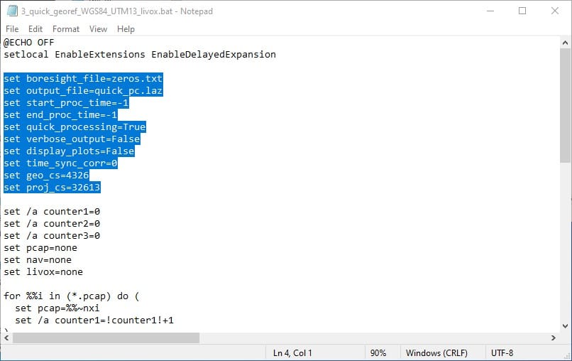
Fig 3.4-9. 3_quick_georef…_livox trigger file (Windows)

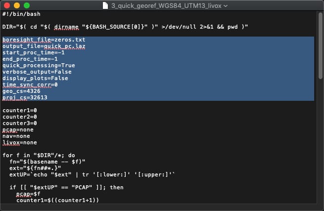
Fig 3.4-10. 3_quick_georef…_livox trigger file (Mac)

The ten processing options for the openmms_georeference_livox.py application are:

1. boresight_file: specifies the ASCII-based file, inside the OpenMMS software installation sys_params subdirectory, that contains the three boresight alignment parameters for the lidar sensor. The default file is zeros.txt. The specified boresight_file can be bypassed if a specially named .bor file is present within the data collection directory (showcased in an upcoming section).

2. output_file: specifies the filename for the point cloud dataset created within the data collection directory. The default filename is quick_pc.laz for the 3_quick_georef…_livox trigger file. Supported output file formats include, .las, .laz, and .csv. IMPORTANT NOTE: If a file with this filename already exists within the data collection directory, it will be overwritten without warning!

3. start_proc_time: specifies the starting timestamp for processing data using UTC seconds within the current day. Any data before this timestamp is ignored. This option supports inline addition and subtraction operators (showcased in an upcoming section). The default value is -1, which indicates processing starts at the beginning of the data.

4. end_proc_time: specifies the ending timestamp for processing data using UTC seconds within the current day. Any data after this timestamp is ignored. This option supports inline addition and subtraction operators (showcased in an upcoming section). The default value is -1, which indicates processing stops at the end of the data.

5. quick_processing: specifies if quick processing should be utilized (True) or not (False). Quick processing only processes 20% of the lidar data collected (1 out of every 5 collected points) from the Livox MID-40 sensor. The default value is True for the 3_quick_georef…_livox trigger file.

6. verbose_output: specifies if the generated point cloud dataset should contain the point attributes needed for the boresight calibration processing (showcased in an upcoming section). The default value is False for the 3_quick_georef…_livox trigger file.

7. display_plots: specifies if a data collection analysis plot, similar to Figure 3.4-4, should be displayed after processing has finished. If set to True, an attempt will also be made to load and display the generated point cloud dataset within the CloudCompare application (be sure to use CloudCompare v2.11 or later, or this functionality may not work correctly). The default value is always False. IMPORTANT NOTE: If this option is set to True, a (potentially) large CloudCompare .bin file also needs to be created inside the data collection directory, thus requiring more computer data storage.

8. time_sync_corr: the .livox ASCII file contains the absolute time instance (in UTC) for the initial Pulse Per Second (PPS) signal that was sent to the Livox lidar sensor. This time reference is vital for synchronizing the lidar data with the trajectory data. There is a very small chance that the time reference reported in the .livox file is incorrect an +1 or -1 integer seconds. This processing option allows a user to adjust the time reference forward or backwards in order to synchronize the lidar data. The default value is 0 (zero).

9. geo_cs: specifies the EPSG number for the geographic coordinate system (i.e., horizontal datum) of the data. The value of 4326 is for the WGS84 datum. Depending on what part of the World the data is from, this option will most likely need to change.

10. proj_cs: specifies the EPSG number for the desired projected coordinate system (i.e., mapping coordinates) of the data. The value of 32613 is for the WGS84 UTM Zone 13 North. Depending on what part of the World the data is from, this option will most likely need to change.

Tip

It helps to create unique trigger files for specific datum and projection combinations that are frequently used. An example being the 3_quick_georef_WGS84_UTM13_livox trigger file used in this demo project.

Execute the third OpenMMS data processing procedure by double-clicking on the 3_quick_georef_WGS84_UTM13_livox file inside the data collection directory. Before execution begins, the 3_quick_georef_WGS84_UTM13_livox trigger file searches its directory for files with the .pcap, .livox, and .txt file extensions. Only a single .pcap file, a single .livox file, and a single .txt file can be present within the directory for execution to start. Error messages will be reported if no .pcap file, .livox file, or .txt file exists or if multiple .pcap files, .livox files, or .txt files exist.

Tip

It usually always helps to turn on the Eye Dome Lighting (EDL) effect within CloudCompare to visualize the point cloud’s features better.

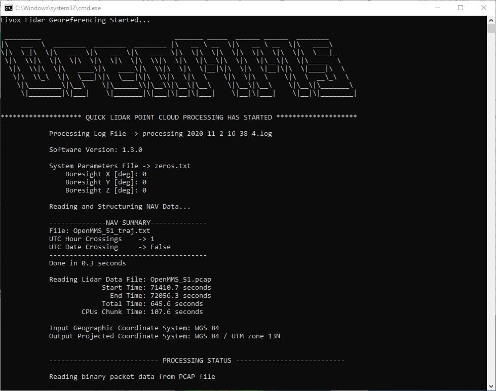
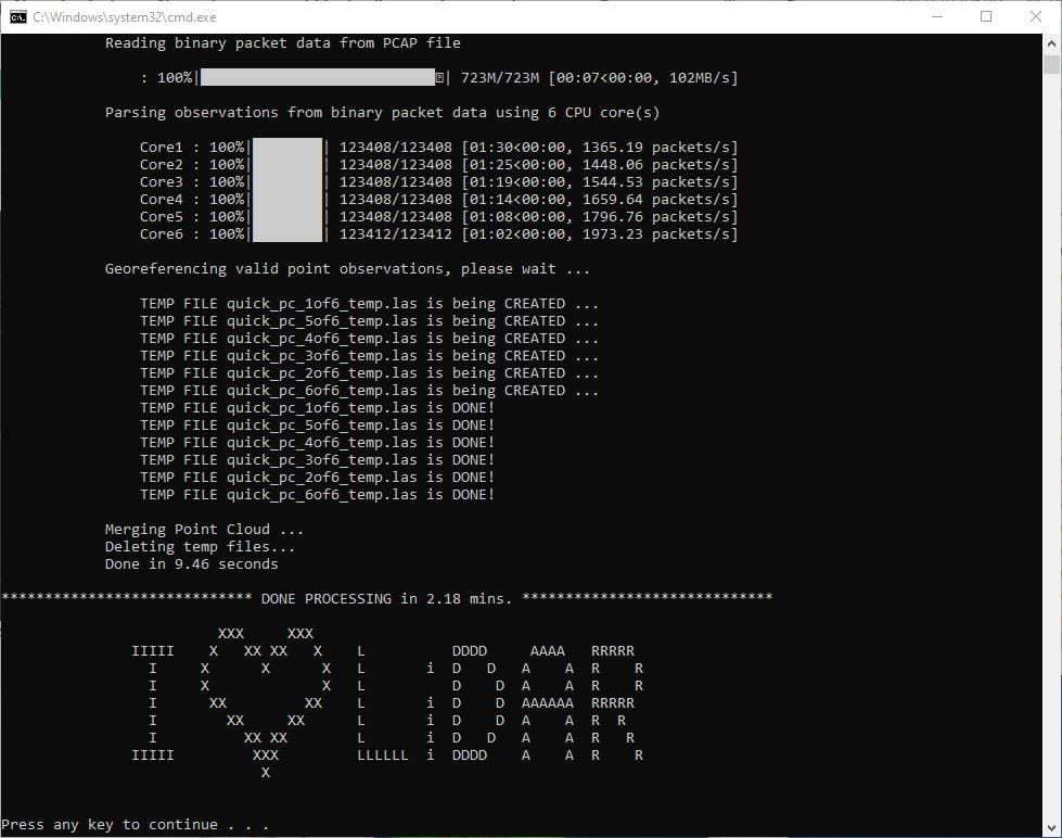
Fig 3.4-11. 3_quick_georef…_livox processing (saved to file)	Fig 3.4-12. 3_quick_georef…_livox processing (multi-core)
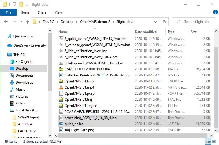
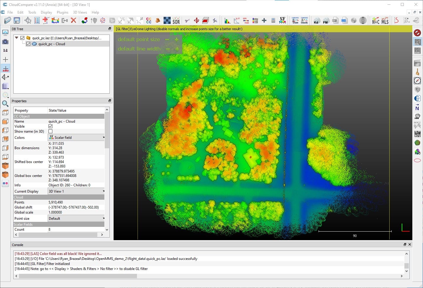
Fig 3.4-13. Directory after executing 3_quick_georef…_livox	Fig 3.4-14. quick_pc.laz being displayed in CloudCompare (w. EDL)

Important

What this documentation calls attributes, CloudCompare calls Scalar Fields (SF).

The processing information displayed within Figures 3.4-11 and 3.4-12 is saved to an ASCII-based .log file within the data collection directory, as shown in Figure 3.4-13. The primary purpose for 3_quick_georef_WGS84_UTM13_livox is to quickly generate a lower accuracy georeferenced point cloud using the collected data, notice the file quick_pc.laz in Figure 3.4-13. Viewing the point cloud’s 3D geometry and attributes within CloudCompare, an understanding of the suitability, or lack thereof, of the collected data can be gained.

Attention

The lower accuracy of the quick_pc.laz point cloud is primarily a result of the position and orientation estimates (a.k.a., trajectory data) within the .traj file being calculated using Standard Positioning Service (SPS) GNSS observations. The highest accuracy trajectory data is produced using a Post-Processed procedure, refer to the following figure.

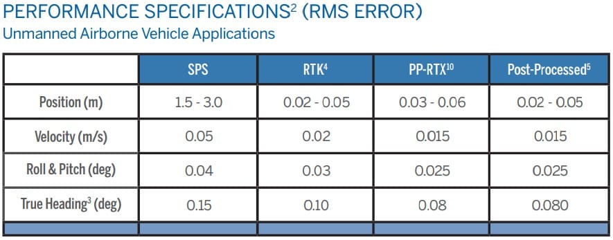
Fig 3.4-15. Applanix APX-18 Performance Specifications (Source: Applanix)

Also, the lidar sensor’s boresight angular misalignment parameters have not yet been estimated. Incorrect values for these parameters can also significantly impact the point cloud’s accuracy. The topic of lidar sensor boresight calibration is discussed in section 3.6.

The accuracy of the point cloud can easily be visualized using CloudCompare (CC). The following video illustrates the steps to perform in CloudCompare to view a cross-section of the point cloud. Notice how the building’s roofline shows several parallel lines of different colored points. The color of the points represents their GpsTime attribute/scalar field (i.e., the different color points were collected at different times during the data collection).

Video 5. Cross section analysis using CC (no audio)

One recommended analysis to perform on the quick_pc.laz point cloud, is to determine the start and stop UTC times for the lidar data of interest (reported as seconds within the day). As an example, OpenMMS Hardware - Section 13.9 explained that the Inertial Navigation System (INS) needs to be initialized before starting data collection. Therefore, the lidar data collected during the initialization period is usually of no interest to the project and can be excluded from further processing. Determining the start and stop UTC times does not have to be performed, but it helps to decrease the file sizes of the generated data and the overall processing time. The following video demonstrates the steps to perform in CloudCompare to determine the start and stop UTC times.

Video 6. Start and stop time analysis using CC (no audio)

Warning

For those readers who are new to using CloudCompare, understanding why and when CloudCompare applies shifts to the geometry or attribute data of a point cloud is vital!

The previous video showed that reasonable estimates for a start and stop UTC times were 52.3s and 607.0s (which in this specific case, is also the end time for the dataset), respectively. However, when opening the quick_pc.laz file within CloudCompare, the GpsTime attributes for all points, were shifted by a constant amount. Therefore, the estimates of 52.3s and 607.0s are incorrect. To discover the magnitude of the shift applied to the GpsTime attribute, the user must either:

1. read the log messages displayed in CloudCompare’s Console interface and find the message that indicates the shift applied to the Time scalar field (see Figure 3.4-16).

2. assign the Active Scalar Field property to GpsTime and use the Point Picking Tool to select any point on the screen. The coordinates message box that appears will show the actual GpsTime attribute value and the shifted value. The magnitude of the shift can then be calculated as the difference between these two values.

The 2nd approach was demonstrated in the previous video. A screenshot showing the GpsTime attribute within the coordinates message box is shown in Figure 3.4-17. Computing the difference yields a shift value of 71433.29s, which agrees with the reported Console message (of course). Therefore, the correct start and stop UTC times would be, 71433.29+52.3 and 71433.29+607.0, respectively.

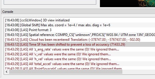
Fig 3.4-16. CC Console showing the applied shift in Time

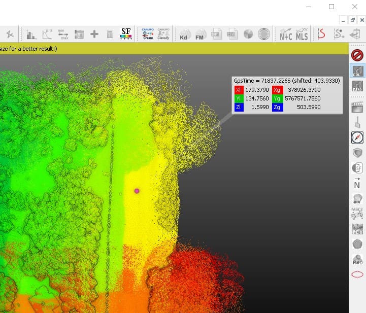
Fig 3.4-17. CC coordinates message box showing Time values

---

3.5 Post-Processed Kinematic (PPK) Trajectory from POSPac UAV

Attention

For those users who do not have access to POSPac UAV software, the two files generated within this section have been included as part of the OpenMMS Demo Project Data. They can be found within the pospac_exports directory.

Note: the event1_eo_5747C00000202010011939_pre_calibration.txt file is the one that is generated within this section.

As discussed in the previous section, the highest accuracy trajectory data is produced using a post-processed procedure. This section demonstrates how to use the Applanix POSPac UAV software to post-process the data in a .T04 file, collected from an Applanix GNSS-INS sensor, along with data in a .T02 file, collected from a Trimble GNSS reference station.

The following summarizes the steps to perform within the POSPac UAV v8.4 SP2 software application:

1. Create a new project using the Livox OpenMMS WGS84 UTM EGM96 template.

2. Save the POSPac project within the data collection directory.

3. Import the .T04 file.

4. Modify Project Settings, the GAMS Standard Deviation will ALWAYS need to be manually set to 1cm.

5. Import the .T02 file (RINEX would also work).

6. Modify the reference station coordinates to precise values, including datum and epoch information.

7. Process GNSS data and review results.

8. Process GNSS and Inertial data.

9. Generate QC Report and review results, especially the Total Body Acceleration and Smoothed Performance Metrics.

10. Export the high accuracy trajectory data to a file, using the OpenMMS_Export format.

11. Generate the Exterior Orientation (EO) data for the camera events, using the OpenMMS_Camera format.

12. Determine the first and last camera event numbers that cover the project area of interest.

13. Save the POSPac project again.

Information

See Video 3 in Tutorial #1 for a demonstration of these thirteen steps.

There are two files created as part of the POSPac UAV post-processing procedure needed before the OpenMMS data processing workflow can continue. These are Auxiliary Files #5 and #6, as discussed previously in section 3.1. The two required files will be named, export_5747C00000202010011939.txt and event1_eo_5747C00000202010011939.txt. These files can be found in the POSPac project directory’s, Export, and EO subdirectories, respectively. Copy these two files into the data collection directory, as shown in Figure 3.5-1. Then move the event1_eo_574…939.txt file into the sony_a6000_images subdirectory, as shown in Figure 3.5-2.

Lastly, for this demo project, the first camera event of interest was 37, and the last camera event of interest was 313. These event numbers are used within section 3.9 below, see Figure 3.9-1.

Warning

Do NOT change the filenames of two required files created using POSPac UAV! Errors in the upcoming processing steps will result.

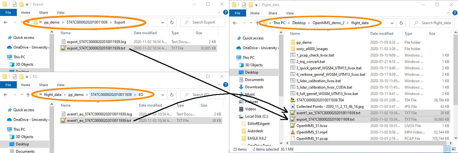
Fig 3.5-1. POSPac UAV generated files copied to data collection directory

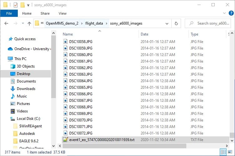
Fig 3.5-2. event1_eo… file moved to sony_a6000_images subdirectory

---

3.6 Lidar Sensor Boresight Calibration

This section presents the second of three calibration procedures that need to be performed on the OpenMMS sensor. Now that the highest accuracy trajectory data has been produced, the lidar sensor’s boresight angular misalignment parameters need to be estimated. There are several published approaches to estimating these parameters. Most, if not all, of the approaches are implemented in-situ rather than in a laboratory environment. An interested reader should have no problem finding vasts amounts of past and present research on this topic. As part of the current OpenMMS data processing workflow, the lidar boresight calibration approach requires the following steps to be performed:

1. Generate a georeferenced point cloud dataset that preserves the lidar observations and high accuracy trajectory parameters for each point.

2. While viewing the georeferenced point cloud using CloudCompare, manually identify unique planar sections (in a wide variety of orientations) and save them to individual files.

3. Execute the 5_lidar_calibration_livox trigger file, which analyzes the individual planar sections and produces a least-squares optimized estimate for the lidar sensor’s boresight angular misalignment parameters. An ASCII-based file will be generated that contains the estimated parameters.

Attention

The OpenMMS lidar boresight calibration approach does NOT require specialized lidar ground targets, or any points, features, or surfaces with known coordinated information to be successfully utilized. For the best results, an area containing lots of precise planar surfaces (with varying normal directions) should be observed by the lidar sensor multiple times and from multiple different directions.

4_VERBOSE_GEOREF

As previously discussed, the 4th trigger file, 4_verbose_georef…_livox, is essentially the same as 3_quick_georef…_livox. The only differences are that the output_file, quick_processing, and verbose_output options are set to different default values. To improve the efficiency of the remaining OpenMMS data processing steps, the previously determined start and stop UTC times can be assigned to the start_proc_time and end_proc_time options within the 4_verbose_georef…_livox trigger file. Be sure to save the trigger file after editing the processing options.

Tip

Remember, that the start_proc_time and end_proc_time processing options support inline addition and subtraction operators. Therefore, their values can be specified as, 71433.29+52.3 and 71433.29+607.0, respectively. Of course they can also be specified as 71485.59 and 72040.29 if desired.

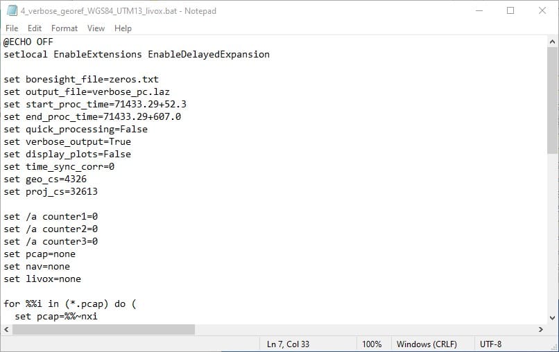
Fig 3.6-1. 4_verbose_georef…_livox file contents

Execute the fourth OpenMMS data processing procedure by double-clicking on the 4_verbose_georef_WGS84_UTM13_livox file inside the data collection directory. Before execution begins, the 4_verbose_georef_WGS84_UTM13_livox trigger file searches its directory for files with the .pcap, .livox, and .txt file extensions. Only a single .pcap file, single .livox file, and a single .txt file can be present within the directory for execution to start. Error messages will be reported if no .pcap file, .livox file, or .txt file exists or if multiple .pcap files, .livox files, or .txt files exist.

Tip

You may receive an error message when attempting to execute the 4_verbose_georef_WGS84_UTM13_livox trigger file. Most likely, this is the result of having two .txt files within the data collection directory. The lower accuracy trajectory file, OpenMMS_51_traj.txt is no longer needed and must be removed or renamed with a different file extension for the execution to start.

The files generated from the execution of the 4_verbose_georef…_livox trigger file are created in the data collection directory and include, an ASCII-based .log file, the georeferenced point cloud with the verbose attributes (named verbose_pc.laz within this demo project), and a new subdirectory named calibration1, see Figure 3.6-4. Within the calibration1 directory, there will be a single .csv file named verbose_offsets.csv. Do not delete or rename this .csv file or errors will occur within upcoming processing steps! Lastly, move the 5_lidar_calibration_livox Trigger File(s) from the data collection directory into the calibration1 subdirectory, see Figure 3.6-5.

Attention

If a subdirectory with the name calibration1 already exists, the 4_verbose_georef…_livox execution will NOT overwrite the subdirectory. Instead, the new subdirectory will be named calibration2, and it will need to be used within the upcoming processing steps. This logic holds for all subdirectories named calibration followed by a number.

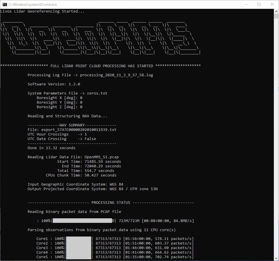
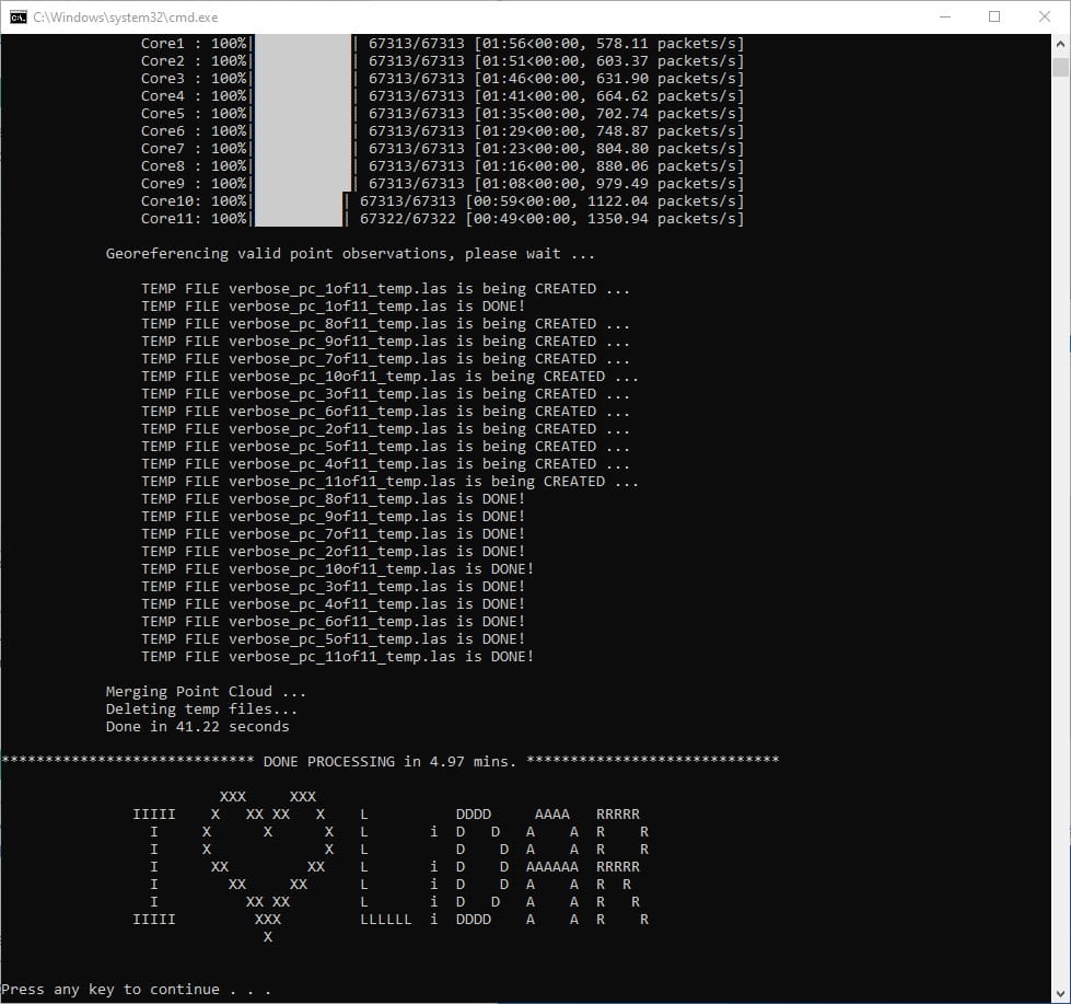
Fig 3.6-2. 4_verbose_georef…_livox processing (saved to file)	Fig 3.6-3. 4_verbose_georef…_livox processing (multi-core)
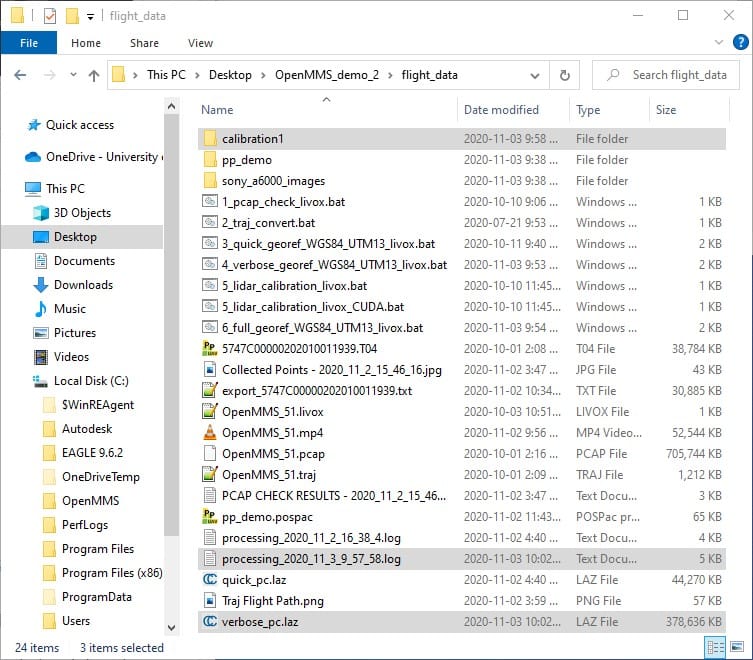
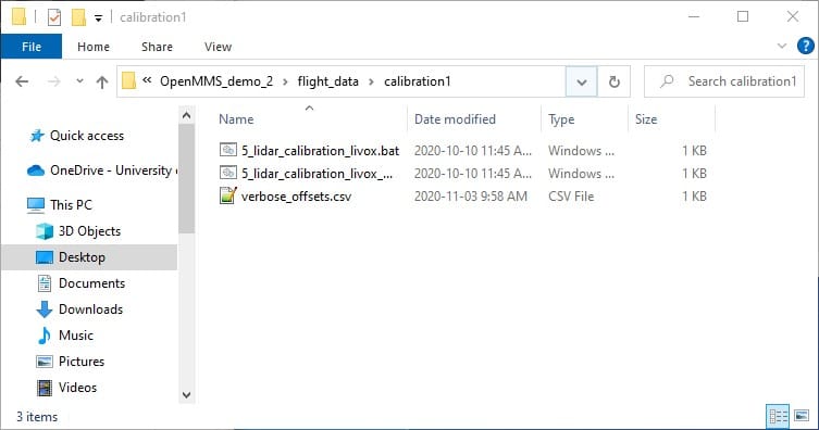
Fig 3.6-4. Directory after executing 4_verbose_georef…_livox	Fig 3.6-5. Move 5_lidar_calibration_livox trigger file(s) to calibration directory

Next, open the verbose_pc.laz point cloud dataset within the CloudCompare software application. Manually identify, select, and clip out planar sections from the point cloud, see Figure 3.6-6 for instructions on how to clip out a smaller section from the overall point cloud. The individual clipped sections should be examined to ensure that the selected points all represent the same planar feature, see Figures 3.6-9 to 3.6-11. Lastly, the planar sections need to be saved to individual ASCII-based .txt files within the aforementioned calibration1 subdirectory, see Figures 3.6-12 and 3.6-13. As previously mentioned, a variety of planar sections with different orientations is ideal.

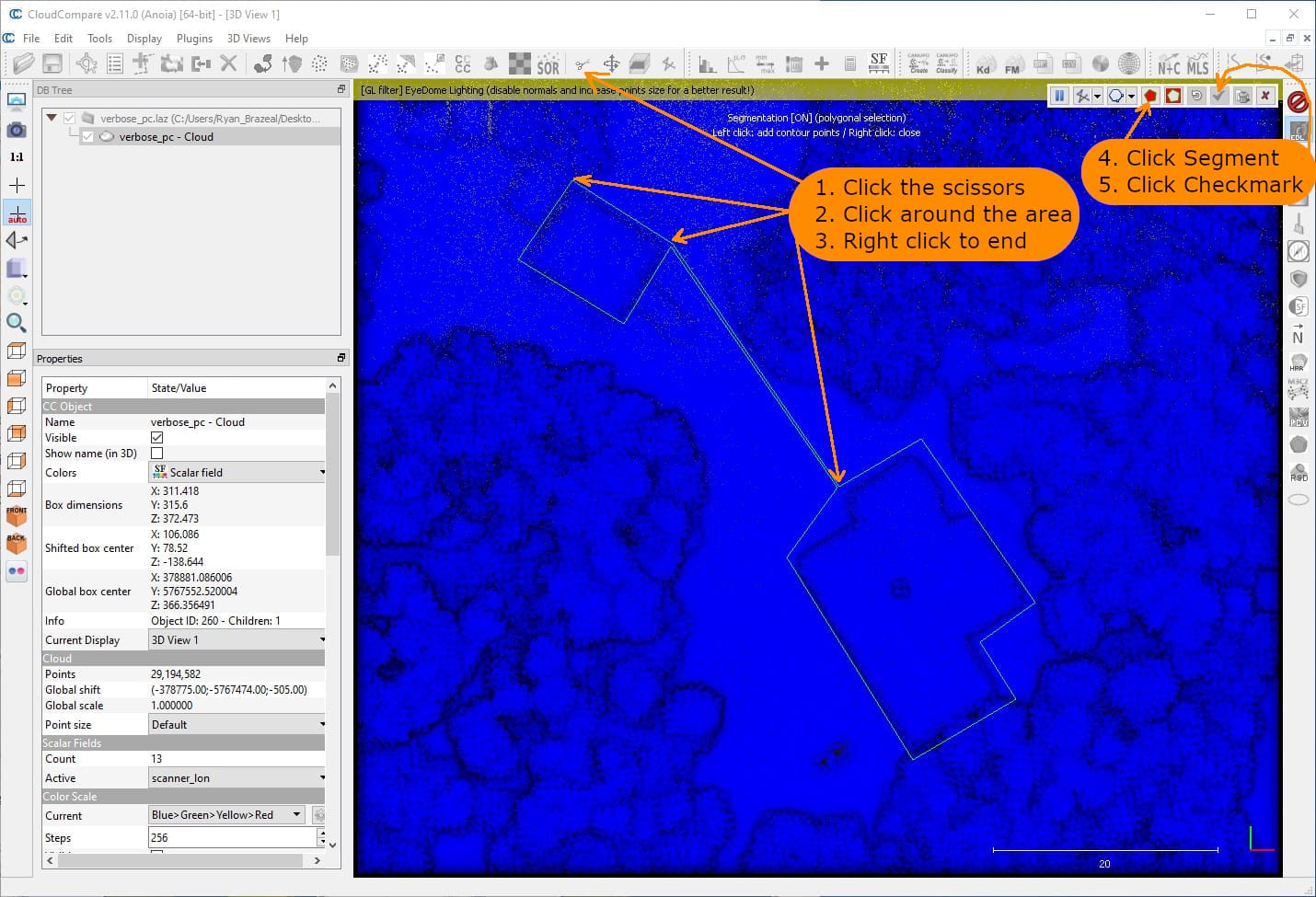
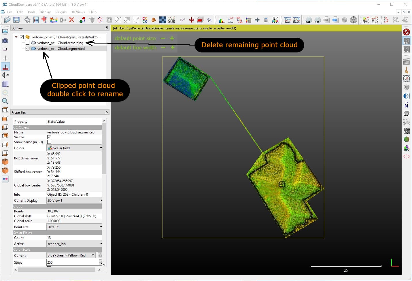
Fig 3.6-6. verbose_pc.laz in CloudCompare (29.1M pts.)	Fig 3.6-7. Isolate buildings with planar features (only 0.4M pts.)
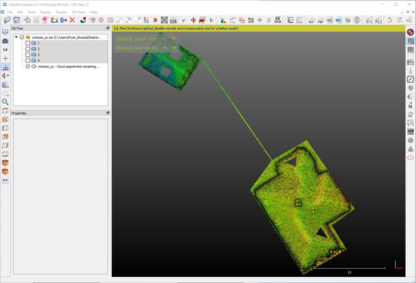
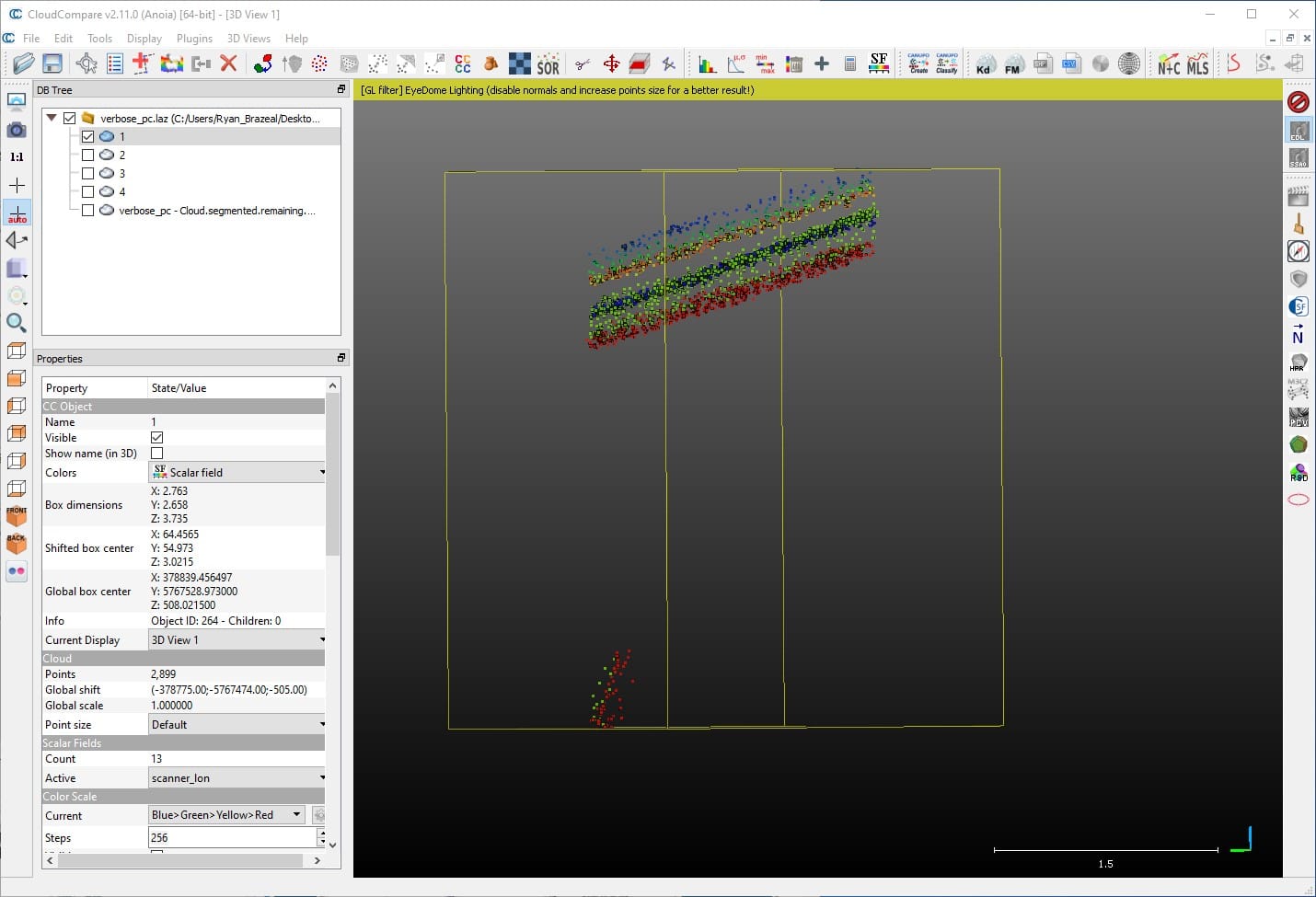
Fig 3.6-8. Clipping 4 small planar sections from the roofs	Fig 3.6-10. Some points in planar section 1 are obviously incorrect
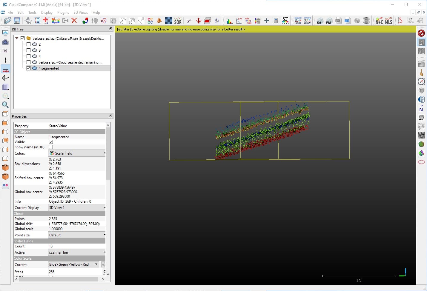
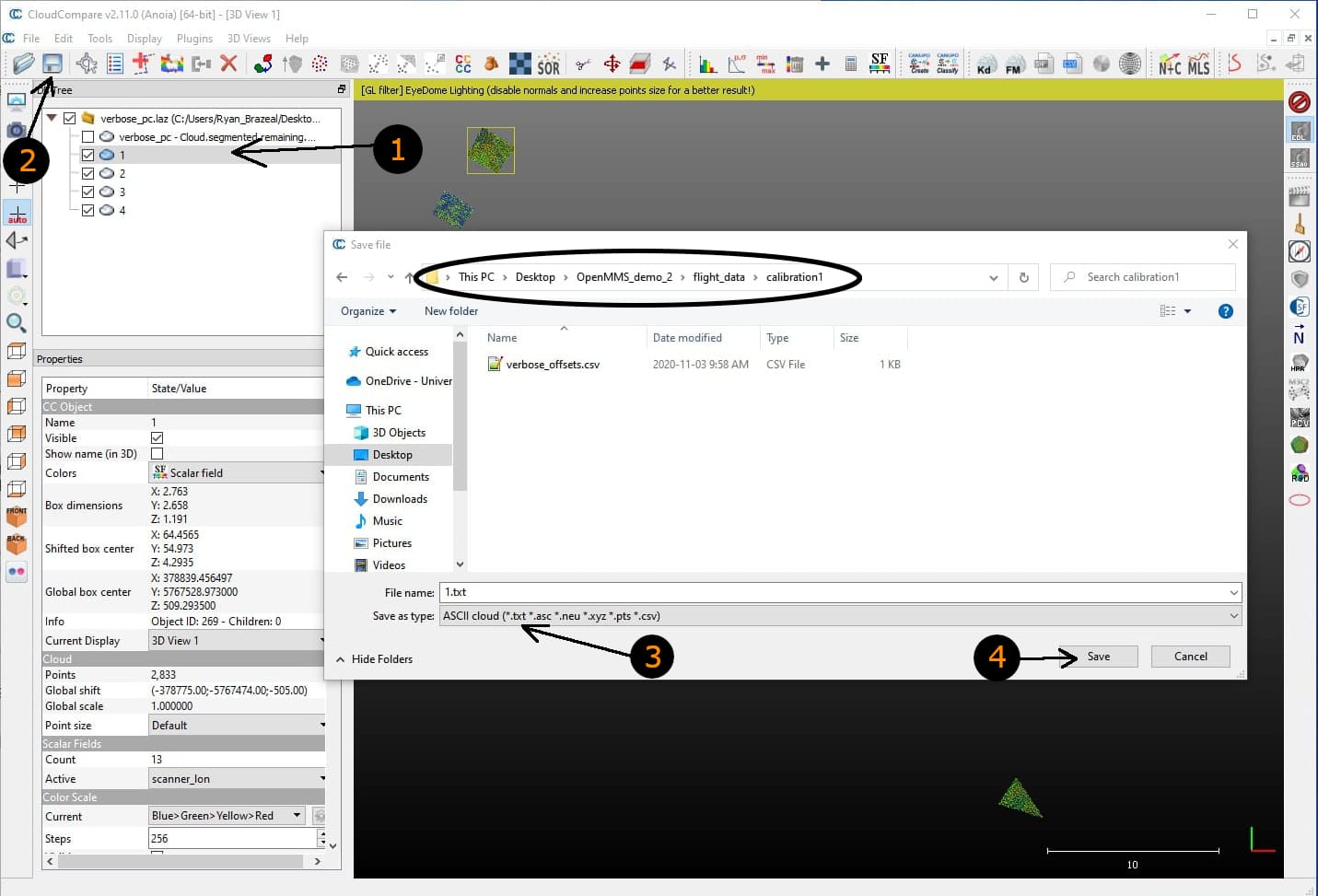
Fig 3.6-11. Planar section 1 is clipped again to remove incorrect points	Fig 3.6-12. Select single clipped section and save it as a .txt ASCII cloud
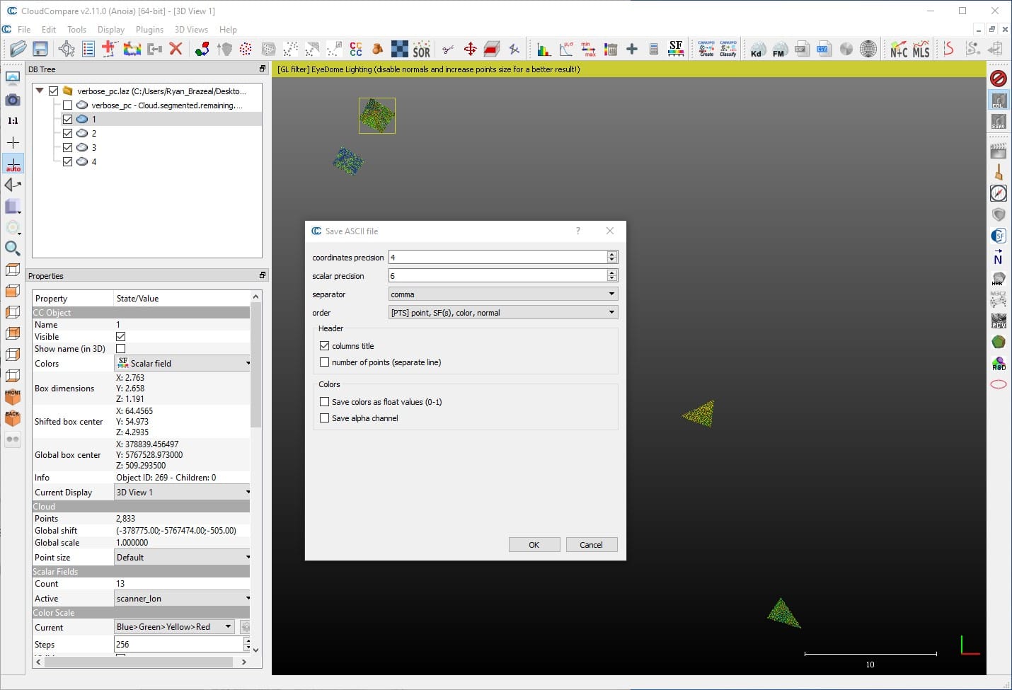
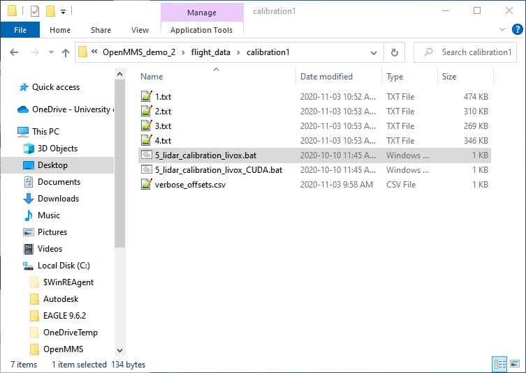
Fig 3.6-13. CC ASCII cloud options (must use exactly as shown)	Fig 3.6-14. The calibration1 subdirectory after clipping planar sections

5_LIDAR_CALIBRATION

Within the 5th trigger file, 5_lidar_calibration_livox, there are NO processing options that can be edited. This trigger file executes the application, openmms_lidar_calibration_livox.py.

Execute the fifth OpenMMS data processing procedure by double-clicking on the 5_lidar_calibration_livox file that is inside the calibration1 subdirectory (or the 5_lidar_calibration_livox_CUDA file, if the user is using a Windows OS based computer that has an NVidia CUDA capable Graphics Card). The application attempts to read the contents of all the .txt files within the calibration1 subdirectory as individual point clouds representing unique planar sections. Figure 3.6-16 illustrates the application’s basic summary information. The benefit of using NVidia CUDA GPU processing is evident when comparing Figures 3.6-17 and 3.6-18. As mentioned, a current development effort is underway to utilize NVidia CUDA GPU processing within as many OpenMMS applications as possible.

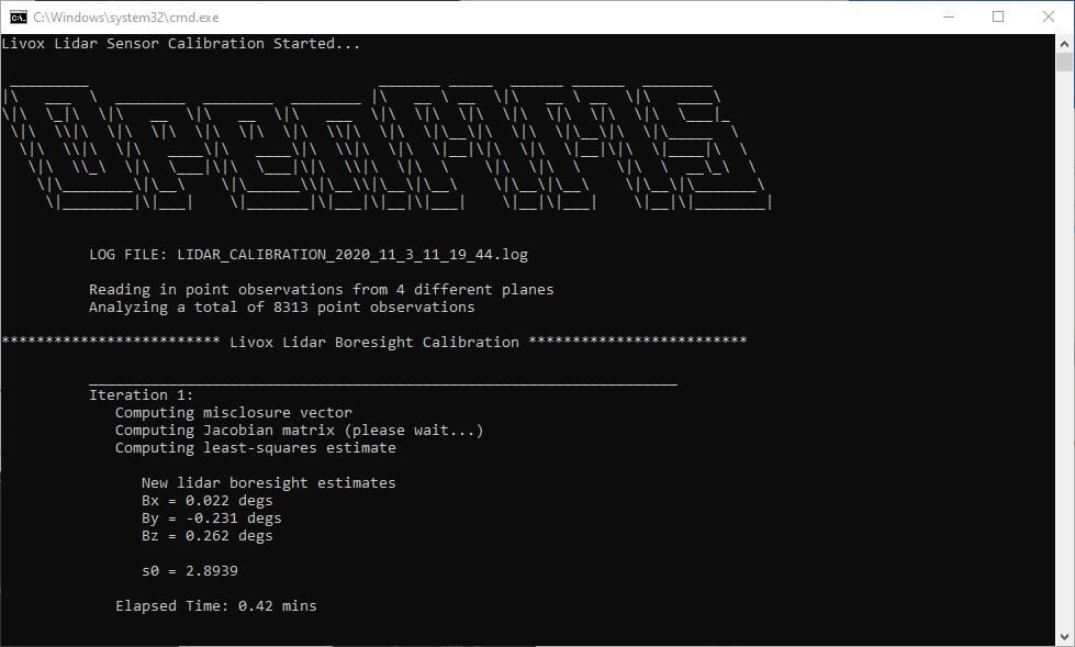
Fig 3.6-16. OpenMMS Lidar Calibration (Livox) summary information (saved to file)

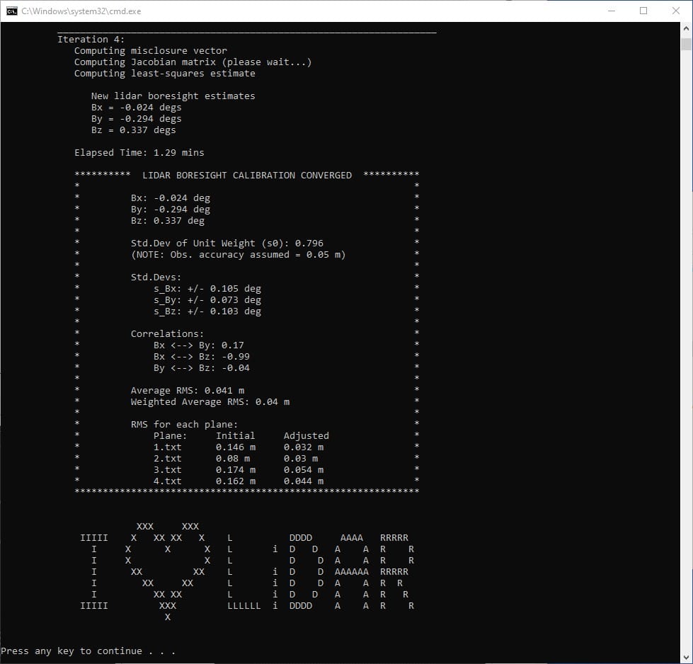
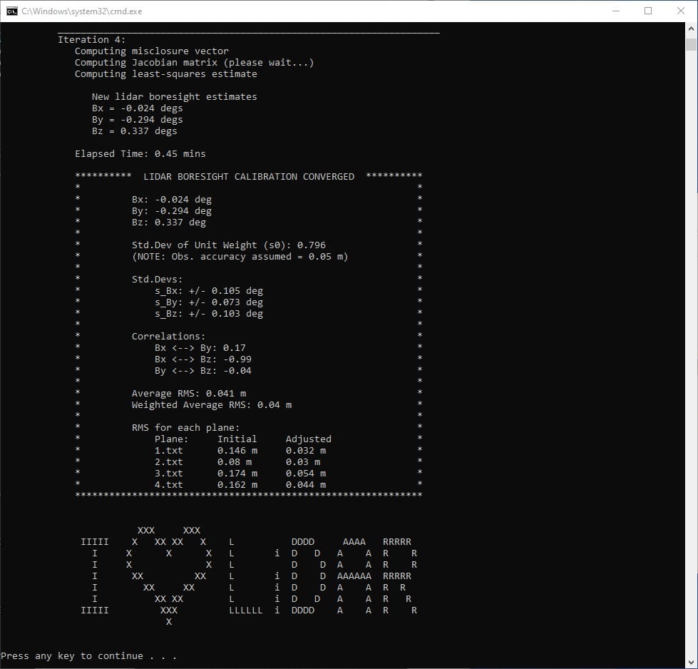
Fig 3.6-17. 5_lidar_calibration_livox results (elapsed time: 1.29 mins)	Fig 3.6-18. 5_lidar_calibration_livox_CUDA results (elapsed time: 0.45 mins)
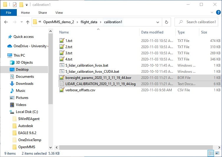
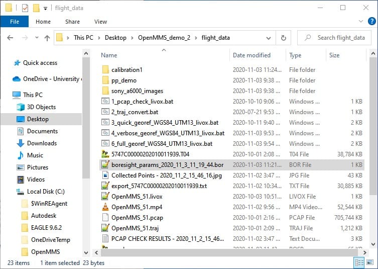
Fig 3.6-19. The calibration1 subdirectory after 5_lidar_calibration_livox	Fig 3.6-20. Lidar boresight estimates .bor file copied to DC dir.

The files generated from the execution of the 5_lidar_calbration_livox trigger file are created in the calibration1 subdirectory and include, an ASCII-based .log file, and an ASCII-based .bor file. The .bor file contains the estimates for the lidar sensor’s boresight angular misalignment parameters. The .bor file will be used within the final lidar georeferencing process, by either:

1. Copying the .bor file into the data collection directory for the current demo project, and all future data collection directories for other projects using the same OpenMMS sensor (assuming the lidar boresight estimates remain constant with time). The openmms_georeference_livox.py application automatically looks for specially named .bor files upon execution and will use the newest file if more than one is found. If a .bor file is found within the data collection directory, it will be used instead of the file specified in the boresight_file processing option.

2. Copying the .bor file into the OpenMMS software installation sys_params subdirectory, and then editing the boresight_file processing option in the trigger files 3, 4, and 6 within the OpenMMS software installation win_batch_files and mac_bash_files subdirectories. Using this approach, all future processing projects will use these edited trigger files, and therefore will use the .bor file.

For this demo project, the .bor file simply needs to be copied to the data collection directory, as shown in Figure 3.6-20.

Warning

Do not change the filename for the generated .bor file, or the lidar boresight estimates may not be applied within the georeferencing processes.

---

3.7 Final Point Cloud Processing & Filtering

With the lidar sensor’s boresight angular misalignment parameters now estimated, the final georeferenced point cloud dataset for the demo project can be generated. The final point cloud is generated using the lidar data, the high accuracy trajectory data, and the lidar boresight estimates. The final processing is executed using the 6_full_georef…_livox trigger file.

6_FULL_GEOREF

As previously discussed, the 6th trigger file, 6_full_georef…_livox, is virtually the same as 3_quick_georef…_livox and 4_verbose_georef…_livox. The only differences are the values set for some of the processing options. To improve the efficiency of the remaining OpenMMS data processing steps, the previously determined start and stop UTC times can be assigned to the start_proc_time and end_proc_time options within the 6_full_georef…_livox trigger file. Be sure to save the file after editing the processing options.

Tip

Remember, that the start_proc_time and end_proc_time processing options support inline addition and subtraction operators. Therefore, their values can be specified as, 71433.29+52.3 and 71433.29+607.0, respectively. Of course they can also be specified as 71485.59 and 72040.29 if desired.

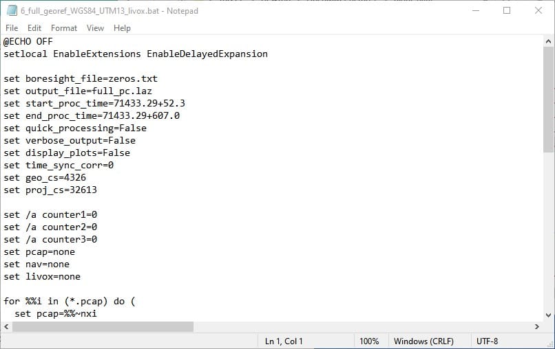
Fig 3.7-1. 6_full_georef…_livox file contents

Execute the sixth OpenMMS data processing procedure by double-clicking on the 6_full_georef_WGS84_UTM13_livox file inside the data collection directory. Before execution begins, the 6_full_georef_WGS84_UTM13_livox trigger file searches its directory for files with the .pcap, .livox, and .txt file extensions. Only a single .pcap file, a single .livox file, and a single .txt file can be present within the directory for execution to start. Error messages will be reported if no .pcap file, .livox file, or .txt file exists or if multiple .pcap files, .livox files, or .txt files exist.

The files generated from the execution of the 6_full_georef…_livox trigger file are created in the data collection directory and include, an ASCII-based .log file and the final georeferenced point cloud (named full_pc.laz within this demo project), see Figure 3.7-3.

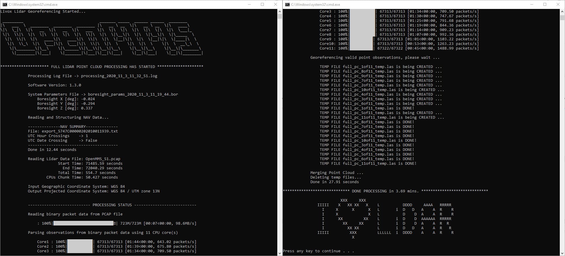
Fig 3.7-2. 6_full_georef…_livox processing results (saved to file)

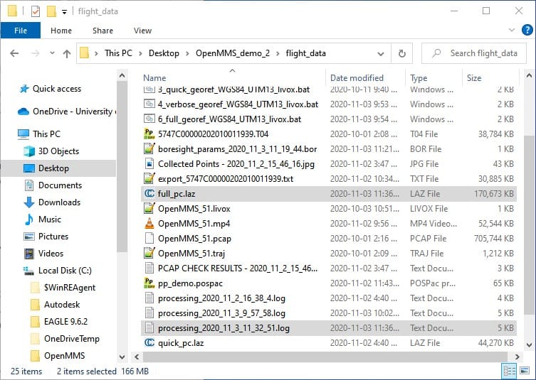
Fig 3.7-3. Directory after executing 6_full_georef…_livox

The last step in generating the final georeferenced point cloud is to open the full_pc.laz file within CloudCompare and remove the unwanted/unnecessary points by filtering based on the point attributes. The following list discusses the eight OpenMMS Extended LAS attributes followed by the three Standard LAS attributes present within the quick and full OpenMMS generated point clouds.

1. scan_azi defines the azimuth angle of the point (within the scanner’s coordinate system). Units are decimal degrees.

2. delta_roll defines the change in the roll orientation angle of the point, with respect to the previously data packet of observed points. This attribute is a remnant of a previous georeferencing approach and no longer plays a vital role in filtering the final point cloud. However, it can still be used to filter out point data observed when the sensor was experiencing quickly changing roll orientation angles during data collection. Units are decimal degrees per second.

3. z_ang_rate defines the lidar sensor’s rate of angular change around the Z axis of the vehicle body frame (i.e., an approximate to the rate of angular change around the direction of the vertical). Similar in usage to the delta_roll attribute, where filtering based on this attribute can eliminate points observed when the sensor was experiencing quickly changing ~heading orientation angles during data collection. Units are decimal degrees per second.

4. v_vel defines the vertical velocity of the sensor when the point was observed. For OpenMMS data collection campaigns from RPAS platforms, this attribute can be used to filter out the take-off and landing time periods (assuming the vertical velocity of the sensor is fairly constant during data collection). Units are meters per second.

5. h_vel defines the horizontal speed of the sensor when the point was observed. This attribute can be used to filter out periods when the sensor was not moving forward, backwards, left, or right, or when the sensor was only rotating (e.g., during stationary turns at the end of RPAS flight lines). Units are meters per second.

6. total_accel defines the absolute value of the total acceleration of the sensor when the point was observed. This atrribute can be used to filter out periods when the sensor was experiencing higher vibrations. Units are g’s (i.e., 1 g = 9.81 m/s^2)

7. heading defines the direction of the sensor when the point was observed. It is important to remember that the sensor is orientated with respect to the vehicle body, such that the side of the sensor where the Sony A6000 camera is mounted (referred to as the Back Face in Hardware documentation), is aligned with the forward/front direction of vehicle body (see section 13.1 in the OpenMMS Hardware documentation for complete details). As a result, the heading attribute is defined as the clockwise angle around the vertical direction with 0 degrees representing the geographical East direction. Units are decimal degrees.

8. range defines the line of sight distance observed from the Livox MID-40 sensor to the point. Many errors are directly proportional to the observed range, so filtering the point cloud based on this attribute can better control the point cloud’s precision. Units are meters.

9. ReturnNumber defines if the point was the first (value = 1) or second (value = 2) observed feature from a single pulse of an observing laser. It is a unitless attribute.

10. GpsTime defines the precise time the point was observed. Units are seconds within the current UTC day. For the special case when the data collection campaign spans across multiple UTC days, the attribute values for the respective points will be greater than 86,400 (i.e., the number of seconds within one day).

11. Intensity defines an 8 bit (0-255) number representing the returned ‘signal strength’ of the transmitted laser pulse. Following the Livox MID-40 documentation, attribute values in the range of 0-150 indicate the observed point is from a non-retroreflective surface, where values >150-255 indicate the observed point is from a retroreflective surface. By filtering based on this attribute, a significant amount of obviously erroneous points can often be removed. It is a unitless attribute.

Important

Because the OpenMMS v1.3 sensor utilizes the triple-return Livox special firmware for the MID-40 sensor, all 2nd return points have a static intensity value of 200 and all 3rd return points have a static intensity value of 250. Read HERE for further details.

The combination of attributes to use to filter the full point cloud and create the final point cloud are not absolute. The attributes that best filter the full point cloud in the desired way(s) are dependent on many different factors. The user is strongly encouraged to experiment with filtering using the different attributes, to better understand the impacts each has. The following figures demonstrate the full point cloud being filtered based on h_vel, and then the results being further filtered by range. Once the filtering has been completed, the resulting point cloud needs to be saved from CC to a file within the data collection directory. For the purposes of this tutorial, the resulting point cloud needs to be saved using the filename, filtered.las

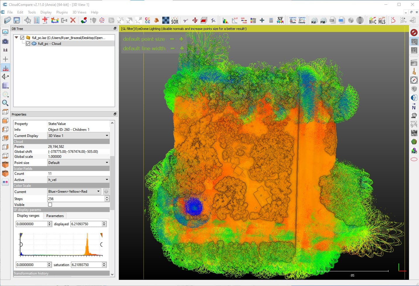
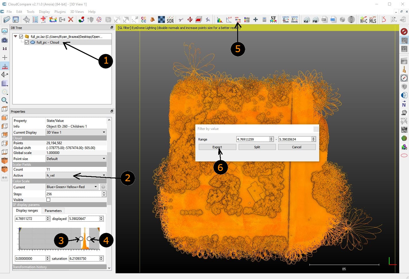
Fig 3.7-4. full_pc.laz colored by h_vel values in CC (29.1M pts.)	Fig 3.7-5. Steps to generate a filtered point cloud in CC
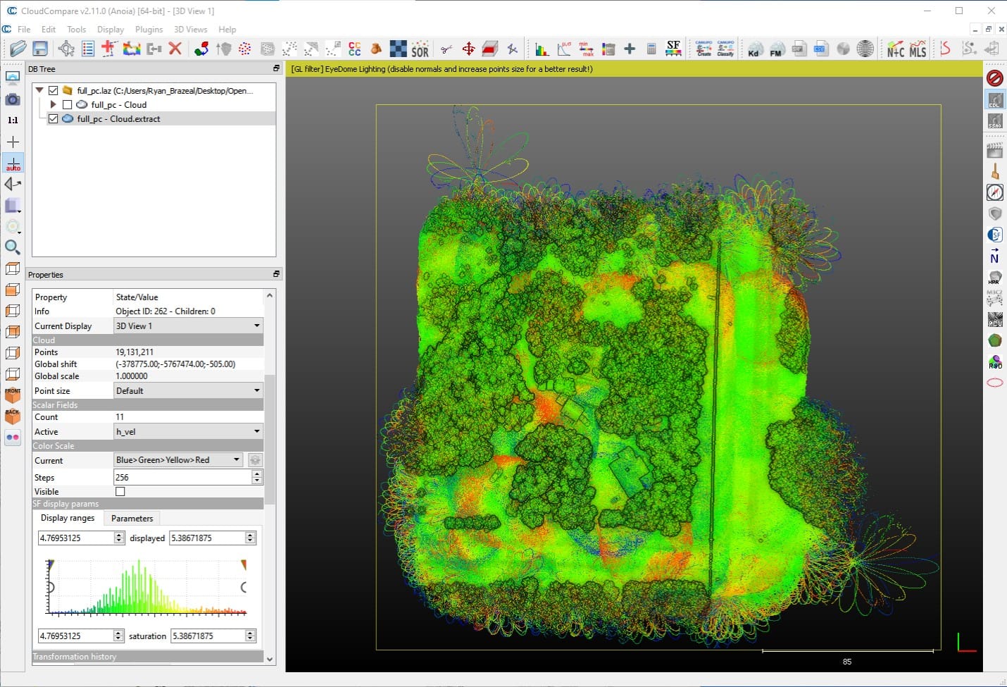
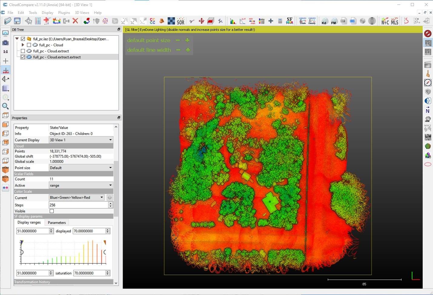
Fig 3.7-6. Results of filtering by h_vel (19.1M pts.)	Fig 3.7-7. Results further filtered by range (18.3M pts.)
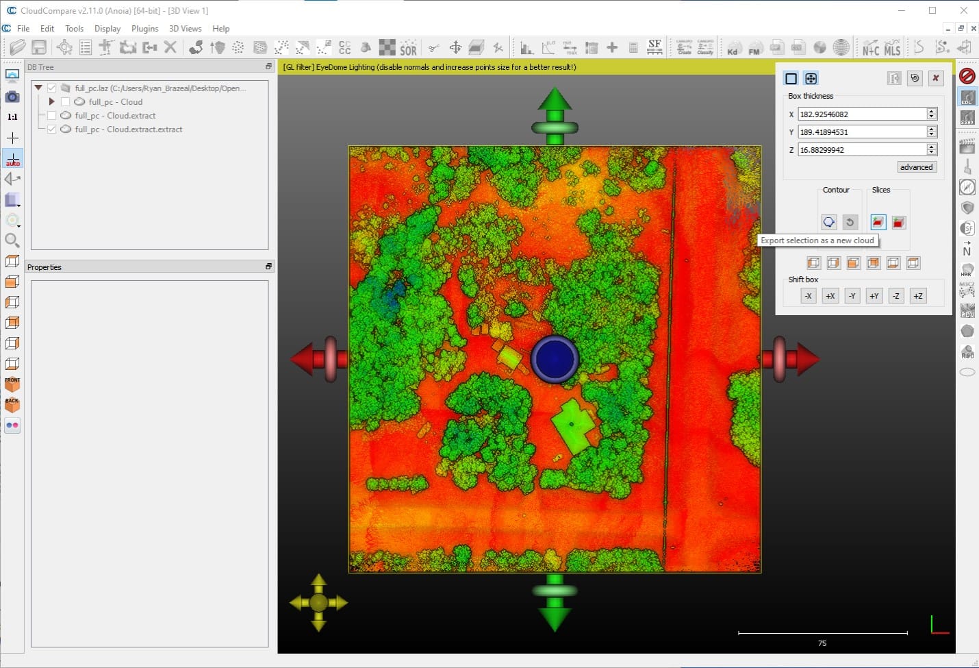
Fig 3.7-8. Use Cross Section tool to ‘square-up’ edges	Fig 3.7-9. Steps to save the filtered.las file in DC dir.

---

3.8 Point Cloud Quality Assurance

The georeferenced point cloud is now in its final state (geometrically speaking). Now is the opportune time to visually and quantitatively assess the spatial accuracy and precision of the OpenMMS point cloud. Begin by opening the filtered.las point cloud within CloudCompare. Next, import the auxiliary dataset #4 (NEH_ground_pts.csv file found within the Demo Project’s gnss_reference_data subdirectory) into CloudCompare. NOTE: the coordinate order for the file NEH_ground_pts.csv is Y, X, Z.

While holding the CTRL key, click the filtered and NEH_ground_pts point clouds within the DB Tree List in CloudCompare. Then, click on the Compute cloud/cloud distance button in the Main tools toolbar. Follow the steps and enter the processing options, as shown in Figure 3.8-2. At this point, the slope distance and the distances in the X, Y, and Z directions between each RTK ground point and their closest respective point within the georeferenced point cloud have been computed. For QA purposes, we are interested in examining the Z distances (i.e., elevation differences) for the RTK points and their closest point cloud estimates. Follow the steps, as illustrated in Figure 3.8-3, to isolate the RTK points and have them colored according to their respective elevation differences. Examine the spatial distribution of the elevation differences across the project area. As a final step, a Gaussian distribution can be best-fit to the sample of elevation differences to visually see if the sample is exhibiting the behavior of a random dataset. The fitted distribution will also report a mean and standard deviation estimate (which are meaningless unless the sample fits a Gaussian distribution).

Attention

It is important to remember, that this analysis is comparing discrete RTK observed points, that were manually identified by a human operator as being on the ground, against points observed by a lidar sensor, that was attached to an RPAS vehicle flying 67 m above the ground and moving at 5 m/s.

Tip

From experience, vegetated areas within the georeferenced point cloud (i.e., a digital surface model - DSM) will likely report more considerable elevation differences to RTK ground points collected within these areas. For best results, the georeferenced DSM point cloud should be further processed to estimate a digital terrain model (DTM) for the project area, and then the DTM should be compared against the RTK ground points. Producing a DTM from a DSM is outside the scope of this documentation.

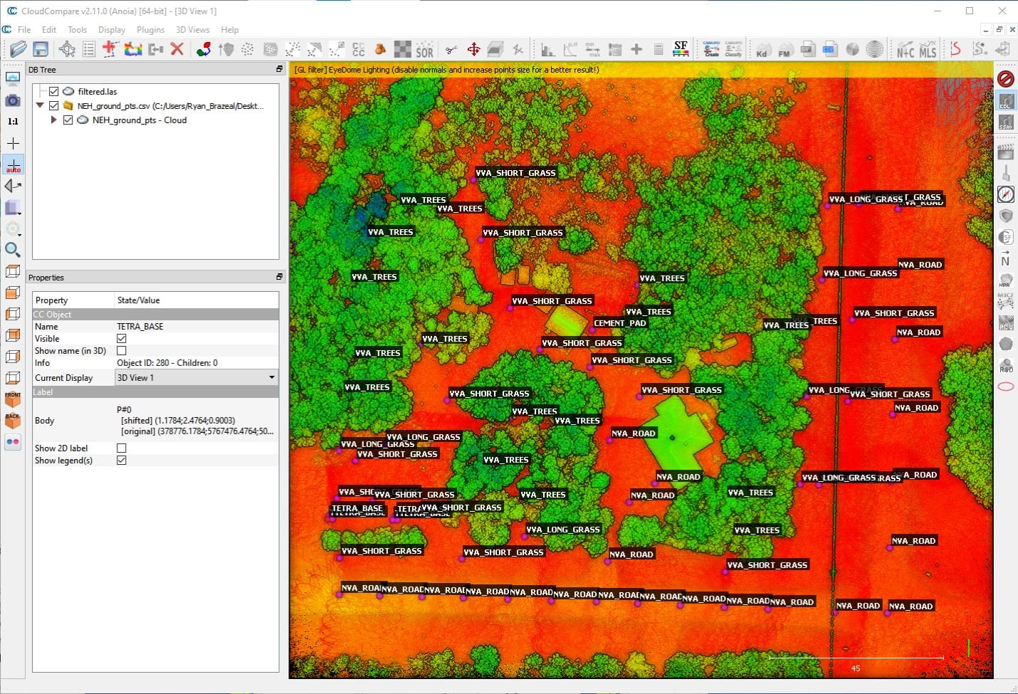
Fig 3.8-1. Filtered point cloud and ground points in CloudCompare	Fig 3.8-2. Steps to perform cloud to cloud comparison in CloudCompare
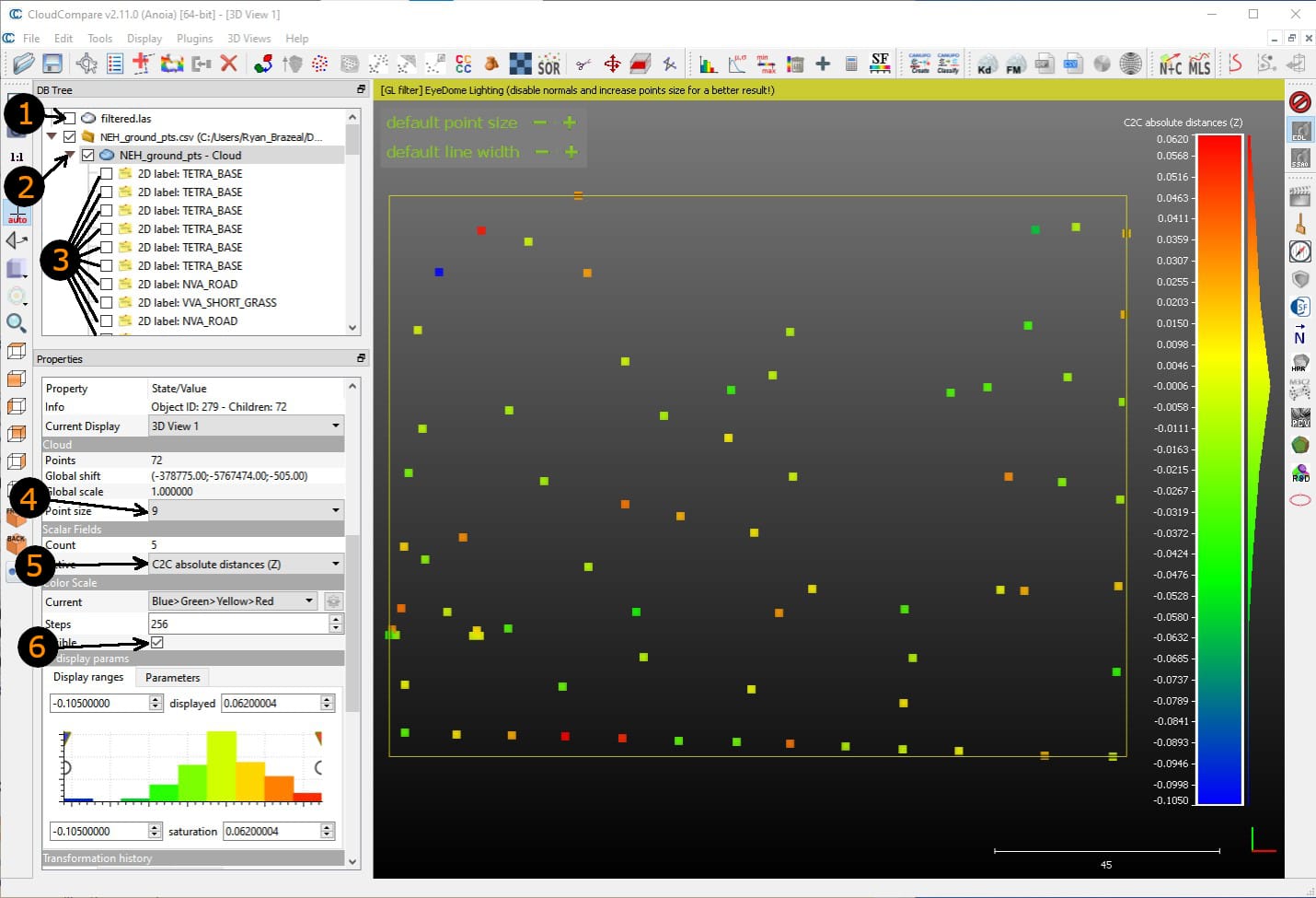
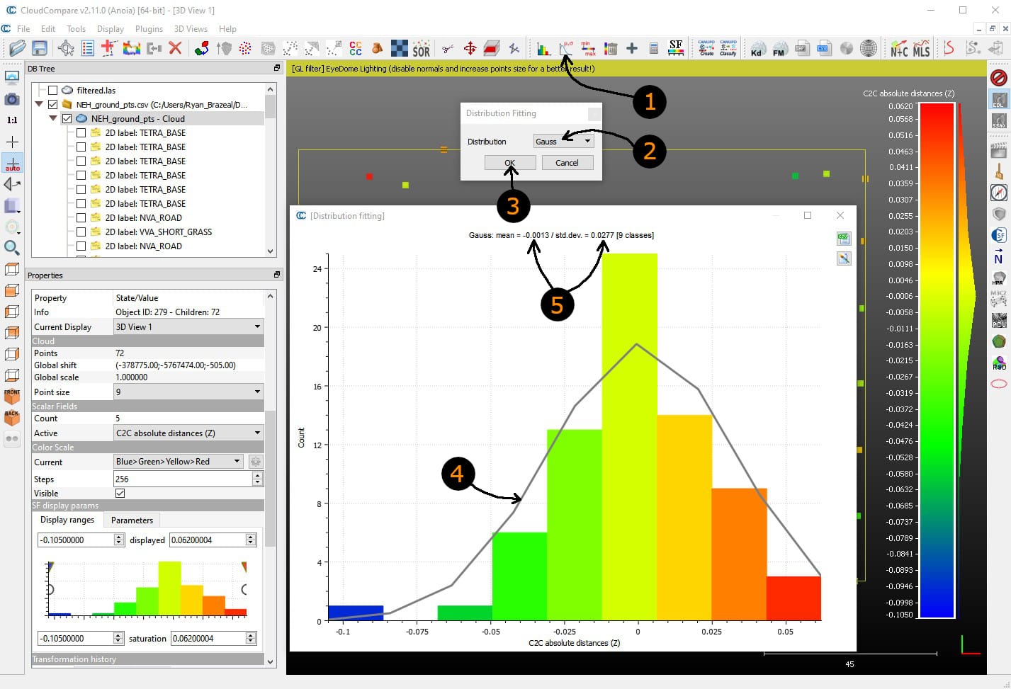
Fig 3.8-3. Ground points colored by height (Z) difference	Fig 3.8-4. Fit Gaussian (normal) distribution to Z differences

---

3.9 Mapping Camera - External Calibration

Attention

The current OpenMMS mapping camera calibration procedure requires using a licensed version of the photogrammetric software, Pix4Dmapper (the free 15-day trial license works perfectly). Future OpenMMS developments also aim to allow the use of Metashape/Photoscan, and OpenDroneMap (ODM) within this camera calibration procedure.

This section presents the last of three calibration procedures that need to be performed on the OpenMMS sensor. The OpenMMS mapping camera calibration procedure can (realistically) only be performed by analyzing MMS data from an RPAS-based data collection campaign. The OpenMMS Sony A6000 Mapping Camera is mounted with its field of view centered around the nadir direction. Therefore, images collected from the sensor while close to the ground will lack the necessary geospatial detail required for the current camera calibration procedure to be effective. The calibration procedure also requires that 3D coordinates (within a realized mapping coordinate system) for a network of pre-surveyed RTK ground control points (GCPs), be known. The ground control points must also be distinguishable within the images collected by the mapping camera.

The final results of this calibration procedure, are the three boresight angular misalignment angles and (optionally) the three lever-arm offsets for the perspective center and optical axis of the mapping camera, with respect to the lidar sensor’s coordinate system. Unlike the lidar sensor’s calibration procedure, these six external calibration parameters need to be re-entered back into the current Applanix POSPac UAV project, and a new exterior orientation (EO) dataset for the collected images needs to be generated and exported. The mapping camera’s external calibration parameters need to be either, re-entered into the settings for every POSPac UAV project, or adjusted within the POSPac UAV project template(s), to be utilized within future OpenMMS projects. In addition to the external calibration parameters, precise estimates for the camera’s interior orientation (IO) parameters are also available from the results of the photogrammetric bundle-block adjustment (BBA) performed by Pix4Dmapper.

Warning

It is well known that the IO estimates for a non-metric camera, generated by a BBA, are usually highly correlated. As a result, the benefit of using the current ‘precise’ IO estimates in future OpenMMS projects may be negligible. That being said, the ‘precise’ IO estimates for a Sony A6000 camera with a Sony 16mm lens are usually not much different than the default IO values. The openmms_preprocess_images.py application (discussed below) also utilizes these default IO values if no other ‘precise’ values are available.

The following discussion outlines how to perform the OpenMMS mapping camera calibration procedure. Start by double checking that the event1_eo… .txt file has been copied from the POSPac UAV Project’s EO subdirectory to the sony_a6000_images subdirectory in the data collection directory, see Figures 3.5-1 and 3.5-2.

7_PREPROCESS_IMAGES

The 7th trigger file, 7_preprocess_images, executes the application openmms_preprocess_images.py. There are NO processing options that can be edited inside this trigger file. Execute this OpenMMS data processing procedure by double-clicking on the 7_preprocess_images file inside the sony_a6000_images subdirectory. This trigger file will be executed a total of three times throughout the OpenMMS data processing. Unlike the other trigger files, the user is prompted to enter the processing options at different times throughout the application’s execution. For the 1st execution of 7_preprocess_images, enter the processing options exactly as shown in the following figure.

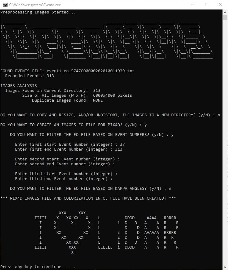
Fig 3.9-1. 7_preprocess_images processing options (1st and 2nd executions)

Warning

It should be noticed that the openmms_preprocess_images.py application determines the number of camera events present within the POSPac generated event1_eo… .txt file, and compares this to the number of .JPG files present within its directory (i.e., the sony_a6000_images directory). These numbers need to match for the processing to continue. The openmms_preprocess_images.py application also analyzes the available metadata for the .JPG files and attempts to determine if any duplicate images are present. If duplicates are detected, the user can instruct the application to move them to a new subdirectory. However, the application cannot (at least currently) detect all the potential issues with the .JPG images and the camera events. Therefore, the user may have to do an additional manual analysis to determine which image corresponds to which camera event. An interested reader should explore POSPac UAV’s Photo ID generation tool, accessible by clicking on the Edit/Create PhotoID File button, as shown in Figure 3.9-6.

Next, create a Pix4Dmapper project and import ALL the Sony A6000 images, the images_pix4d.csv file (generated in the previous step, see Figure 3.9-2), and the NEH_ground_control_pts.csv file found in the demo project’s gnss_reference_data subdirectory. Video 4 in tutorial #1 demonstrates how to use Pix4Dmapper to generate the auxiliary files needed to perform the OpenMMS camera calibration. Pay close attention to all the steps as well as the textboxes within the video. Upon completion of the Pix4Dmapper processing, copy the two generated files (i.e., auxiliary files #8 and #9) from the Pix4D project folder -> 1_initial -> params to the sony_a6000_images subdirectory, see Figure 3.9-3.

Attention

For those users who do not have access to Pix4Dmapper software, the two files generated within this section have been included as part of the OpenMMS Demo Project Data, and can be found within the pix4d_exports directory.

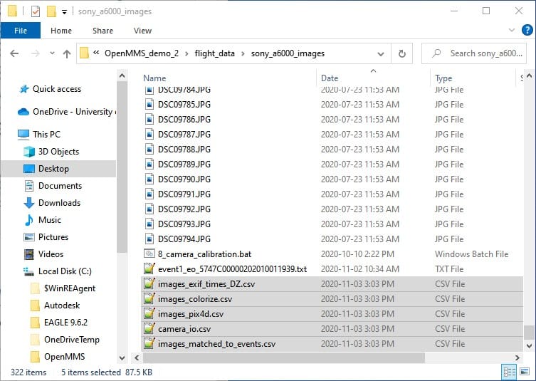
Fig 3.9-2. Results of 7_preprocess_images in subdir.

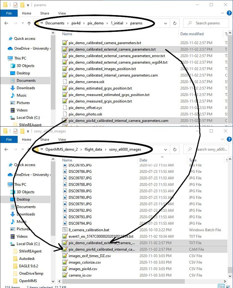
Fig 3.9-3. Pix4D generated files copied to sony_a6000_images subdir.

8_CAMERA_CALIBRATION

The OpenMMS mapping camera external calibration can now be performed. The eighth trigger file, 8_camera_calibration, executes the application openmms_camera_calibration.py and contains two processing option that can be edited. To begin, open the 8_camera_calibration file using a text editor (do not double click on it). The following figure illustrates the one processing option within the trigger file on Windows OS.

Fig 3.9-4. 8_camera_calibration trigger file contents (Windows)

The two processing options for the openmms_camera_calibration.py application are:

1. max_images: this option specifies the maximum number of images used within the camera calibration mathematical analysis. If max_images is less than the total number of images available, then a subset of the total images is used. The sampling is evenly spaced (as much as possible) from the available images. The default value is 500 images.

2. orientation_only: this option specifies if only the boresight calibration parameters are to be estimated. If orientation_only is set to False, then the lever arm offset values between the origin of the lidar sensor and the perspective center of the camera will also be estimated. The boresight estimates and lever arm estimates are usually very highly correlated. The default value is True.

Execute the 8_camera_calibration trigger file by double-clicking on the file inside the sony_a6000_images subdirectory. The OpenMMS camera calibration procedure performs a least-squares analysis using the observed EO data exported by POSPac UAV, and the control EO data produced by the bundle-block adjustment within Pix4Dmapper. The camera’s external calibration parameters are optimized to minimize the differences between the observed EO data with respect to the control EO data. The results of the camera calibration procedure are displayed directly within the command-line interface dialog (see the blue box in Figure 3.9-5), as well saved to an ASCII-based .log file within the sony_a6000_images subdirectory.

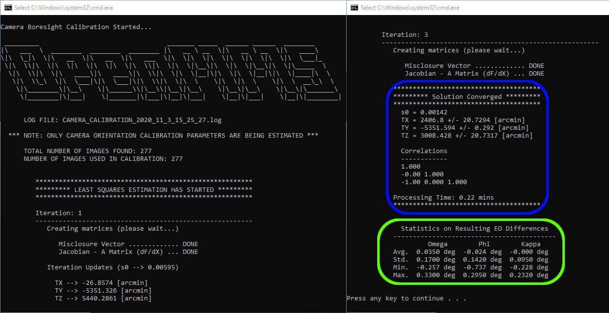
Fig 3.9-5. 8_camera_calibration execution results (saved to .log file)

Next, the camera calibration parameters need to be copied and entered into the POSPac UAV software within the Project Settings -> Camera -> Lever Arms, Boresights and Photo ID -> Reference to Camera Lever Arm and Reference to Camera Boresight Angles sections, see Figure 3.9-6. Re-export the EO dataset for the camera events (which produces the needed auxiliary file #7) by selecting the Tools tab in the POSPac UAV menubar and clicking the Exterior Orientation Processor button, see the 5:38 timestamp of Video 3 in tutorial #1 for clarification. Next, the re-exported event1_eo… .txt file, found in the POSPav UAV Project’s EO subdirectory, needs to be copied to the sony_a6000_images subdirectory, see Figure 3.9-7.

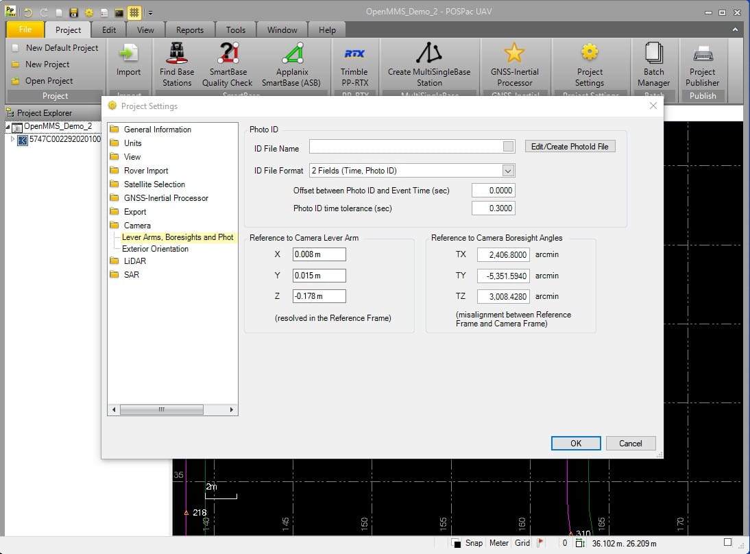
Fig 3.9-6. POSPac Project Settings for camera calibration parameters

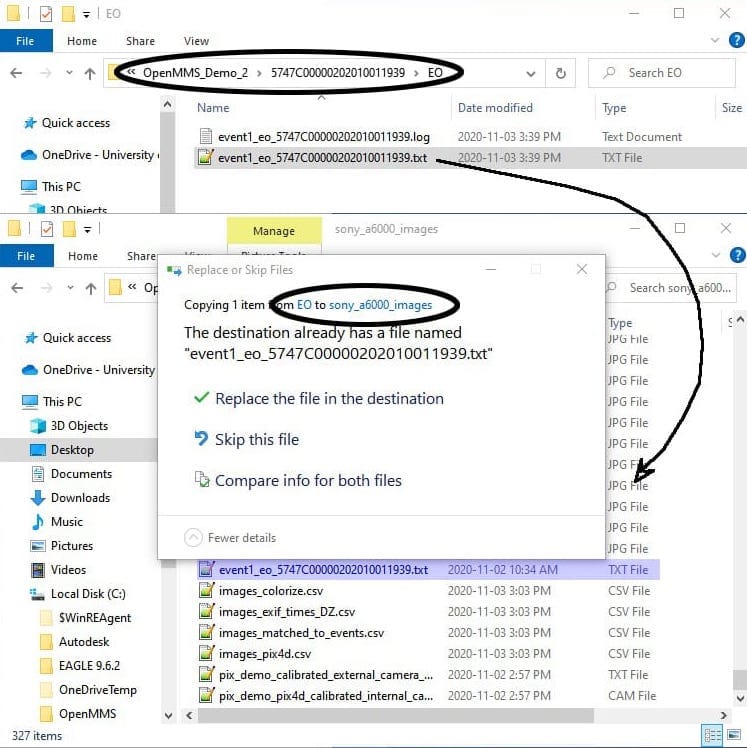
Fig 3.9-7. Update event1_eo… .txt file in sony_a6000_images subdir.

The OpenMMS camera calibration is now complete! However, a few additional processing steps are strongly recommended as a Quality Assurance measure. First, the 7_preprocess_images trigger file needs to be executed for the 2nd time. Enter the processing options exactly as shown in Figure 3.9-1. This processing will produce a new images_pix4d.csv in the sony_a6000_images subdirectory.

Reopen the Pix4Dmapper project, and open the Image Properties Editor dialog, see Figure 3.9-8. Click the Clear button to remove the previous EO parameters (i.e., X, Y, Z, Omega, Phi, Kappa). Click the From File… button. Within the Select Geolocation File dialog that appears, select the X,Y,Z File Format. Browse to the new images_pix4d.csv file and select it. Close the open dialogs by clicking either the Open or OK button.

Fig 3.9-8. Pix4Dmapper Image Properties Editor dialog

Open the GCP/MTP Manager dialog, see Figure 3.9-9. Click anywhere within the first row of the table to select the GCP. While holding the SHIFT key, click anywhere within the last row of the table to select ALL the GCPs. Right-click anywhere within the Type column and select Edit Types in Selected Rows. Change all the GCPs to the Check Point type. Click OK to save and close the dialog.

Fig 3.9-9. Pix4Dmapper GCP/MTP Manager dialog

Click the Processing Options button in the bottom-left corner of the Pix4Dmapper application. On the Processing Options dialog that appears (see Figure 3.9-10), select the 1. Initial Processing item from the list, and select the Calibration tab. Change the Calibration Method from Standard to Accurate Geolocation and Orientation. Before clicking the OK button, make sure that ONLY the 1. Initial Processing item is checked, and the other two items are NOT checked.

Fig 3.9-10. Pix4Dmapper Processing Options dialog

Once the edits to the images’ EO parameters, the GCPs’ types, and the processing options have been made, the Pix4Dmapper project needs to be Reoptimized. From the main menu at the top of the Pix4Dmapper application, select the Process menu, and click on Reoptimize. It is ok to overwrite the previous processing results when prompted. Once the progress bar near the bottom-left corner of the application reports Done, Regenerate Quality Report from the menu, if needed., the final step is to click on Generate Quality Report from the Process Menu. Once the Quality Report has been generated, it will be automatically displayed on the screen.

Examine the Geolocation Details section near the end of the report. Within the Ground Control Points section, the Mean [m] values for the Errors in X, Y, Z should all be nearly zero, and the Sigma [m]/RMS Error [m] values should all be 2-5cm (ideally), see Figure 3.9-11. This analysis represents the positional error witnessed on the ground at the locations of the GCPs. Within the Absolute Geolocation Variance section, a tabular error distribution for the Errors in the X, Y, Z coordinates of the images is presented, see Figure 3.9-12. Ideally, these distributions should closely conform to a Gaussian distribution. This analysis represents the positional error witnessed at the camera locations, and not on the ground. Lastly, the Geolocation Orientational Variance table discusses the Euler rotation angles (e.g., Omega, Phi, Kappa) that define the direction of the camera’s optical axis when each image was taken. The RMS [degree] values for each angle, based on the differences between the initial POSPac EO data and the BBA EO data, are presented. Ideally, these values should be very close to the boresight estimates from the camera calibration procedure (examine the values in the yellow box in Figure 3.9-5).

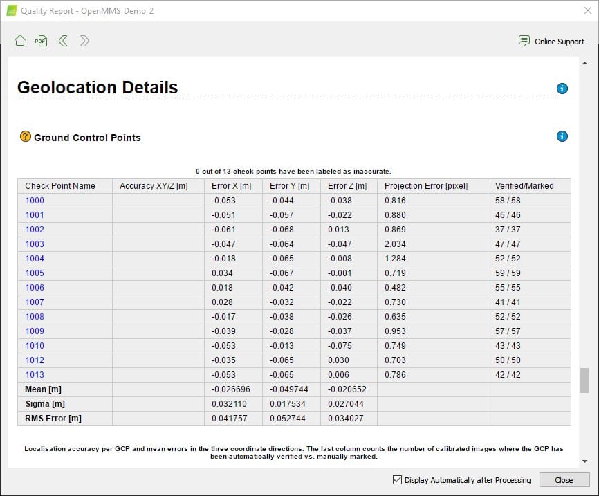
Fig 3.9-11. Geolocation Details - GCPs

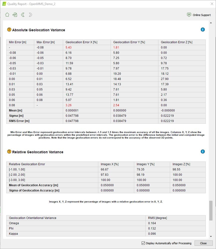
Fig 3.9-12. Geolocation Details - Position and Orientation Differences

---

3.10 Point Cloud Colorization

It was essential to develop and include a rigorous point cloud colorization solution within the currently offered OpenMMS suite of open-source software applications. The OpenMMS point cloud colorization procedure offers several processing options. The options allow for the real-world color of a lidar observed point to be determined using:

1. The mapping camera image that was taken at the time epoch closest to when the point was observed.

2. The mapping camera image that was taken at the position closest to the observed point.

3. A balanced (i.e., blended) color computed using up to three of the closest mapping camera images (based on time or position).

The OpenMMS point cloud colorization procedure utilizes the perspective geometric relationship between the lidar observed points and the mapping camera images to determine which image pixel corresponds to each lidar observed point. Therefore, an orthorectified mosaic is not utilized within the OpenMMS point cloud colorization procedure. Using perspective imagery within the colorization procedure allows for features that would be occluded within orthorectified imagery to be colorized more rigorously.

Begin the OpenMMS point cloud colorization procedure by executing the 7_preprocess_images trigger file for the 3rd (and final) time. Enter the onscreen processing options exactly as shown in Figure 3.10-1.

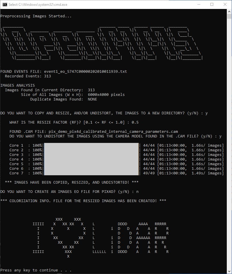
Fig 3.10-1. 7_preprocess_images processing options (3rd execution)

The result of this processing step is the creation of a new subdirectory within the sony_a6000_images directory, named resized_X.Y, see Figure 3.10-2. Within the resized_X.Y subdirectory, copies of all of the original mapping camera images resized by the factor * X.Y* are generated. Additionally, the user can select if the original images should also be undistorted based on either, the ‘precise’ IO parameters estimated within the Pix4D processing (made available via the .cam file), or the default set of IO parameters for a Sony A6000 camera (with 16mm lens). Lastly, the 9_colorize_las trigger file needs to be moved from inside the sony_a6000_images directory, and put inside the new resized_X.Y subdirectory, see Figure 3.10-3.

Tip

It is strongly recommended to resize the original images by a minimum value of 0.5 and undistort the images based on either a .cam file or the default values. By resizing and undistorting the images the colorization procedure will be more computer memory friendly, faster, and the colorization results will still be excellent!

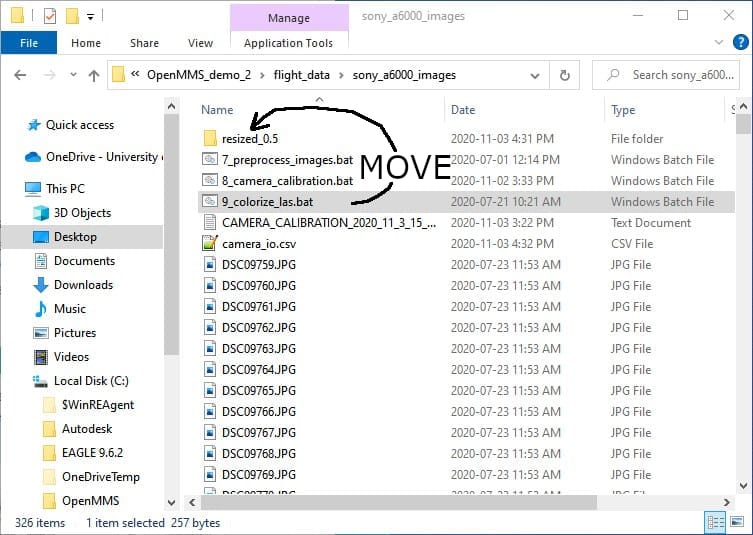
Fig 3.10-2. New resized_X.Y subdirectory

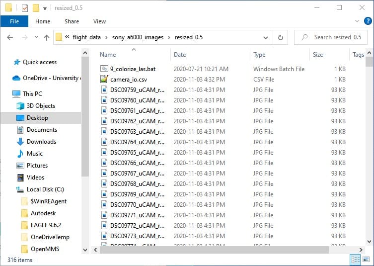
Fig 3.10-3. Contents of the new resized_X.Y subdirectory

9_COLORIZE_LAS

The OpenMMS point cloud colorization procedure can now be performed. The ninth trigger file, 9_colorize_las, executes the application openmms_colorize.py and contains three processing options that can be edited. To begin, open the 9_colorize_las file using a text editor (do not double click on it). The following figure illustrates the three processing options within the trigger file on Windows OS.

Fig 3.10-4. 9_colorize_las trigger file contents (Windows)

The three processing options for the openmms_colorize.py application are:

1. las_file: this option specifies the relative path, from the current directory, and filename for the .las point cloud file to be colorized. The default value is ..\ ..\filtered.las (Windows) or ../../filtered.las (Mac/Linux) which indicates that the .las file to be colorized is named filtered.las and it exists within the grandparent directory (i.e., up 2 hierarchy levels from the current directory).

Warning

Windows OS uses \ characters within path strings, while Mac OS and Linux distros use / characters. Be careful to use the correct syntax.

2. color_balance: this option specifies the number of closest images (time-based or distance-based) to be used to compute the balanced color for each observed point. The default value is 1 (valid options are 1-3 inclusive).

3. do_dist_search_after: this option specifies if a secondary distance-based colorization procedure should be performed after the primary time-based colorization procedure has completed. Only the remaining uncolored points will be analyzed within the secondary colorization procedure. The default value is False.

Execute the 9_colorize_las trigger file by double-clicking on the file inside the resized_X.Y subdirectory. The result of the point cloud colorization procedure is a new colorized .las point cloud file generated within the same directory as the specified las_file processing option. IMPORTANT NOTE: it is possible that the new colorized point cloud dataset will be saved as multiple .las files. This attempts to fix an odd 32 bit issue that was experienced during development. A notice message near the top of the command-line dialog for the point cloud colorization procedure will alert the user if multiple .las files will be created, see Figure 3.10-5.

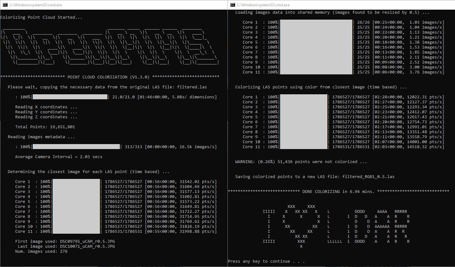
Fig 3.10-5. 9_colorize_las execution results (using default processing options)

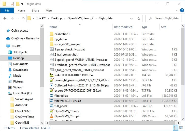
Fig 3.10-6. New colorized .las point cloud file(s)

The new file(s) can be opened within CloudCompare to view the colorized point cloud and merge the multiple point clouds into a single .las (or other) point cloud file format, if desired. An OpenMMS colorized point cloud contains two additional point attributes (i.e., scalar fields in CloudCompare). The two attributes are:

1. image_used: this specifies the index number of the image used to colorize the point. The index numbers start at 1 for the first mapping camera image. A value of 0 indicates that no mapping camera image was found that contained the point. By filtering based on this attribute, the user can isolate a subset of the point cloud that covers the field of view of a specific mapping camera image for further investigation or research purposes.

2. color_class: this specifies the color class number for the point. A value of 0 indicates that the point has not been colorized. A value of 1 indicates that the point was colorized using the closest time-based image(s). Lastly, a value of 2 indicates that the point was colorized using the closest distance-based images(s). By filtering based on this attribute, the user can isolate only the colorized (or uncolorized) points within the entire point cloud, see the figures below.

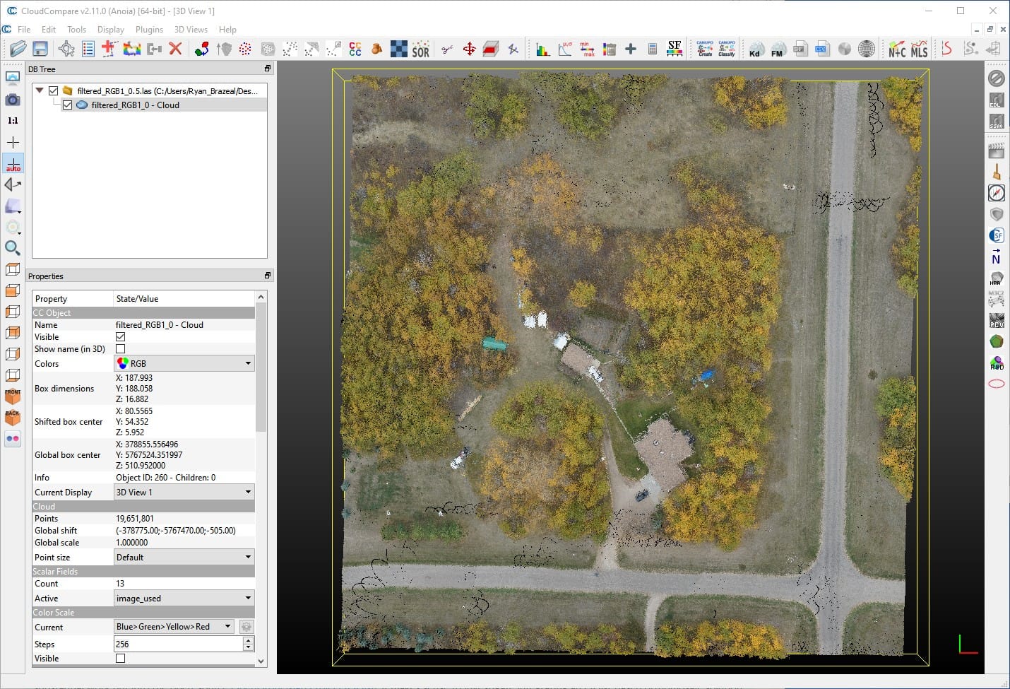
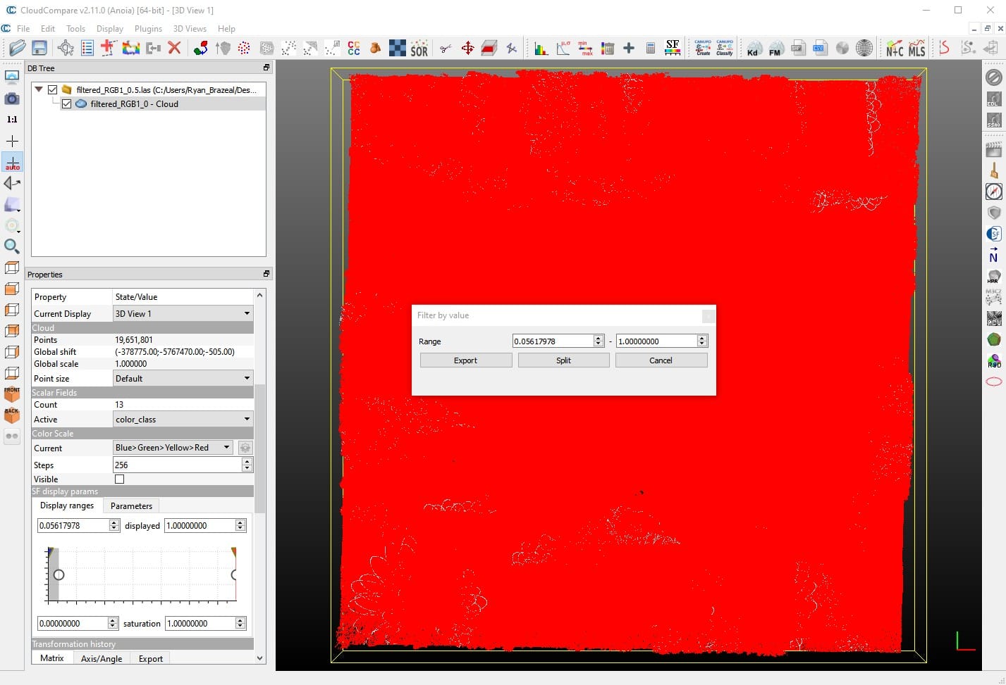
Fig 3.10-7. Colorized point clouds with mixed color classes	Fig 3.10-8. Filtering the color class to values > 0 (i.e., colored pts.)
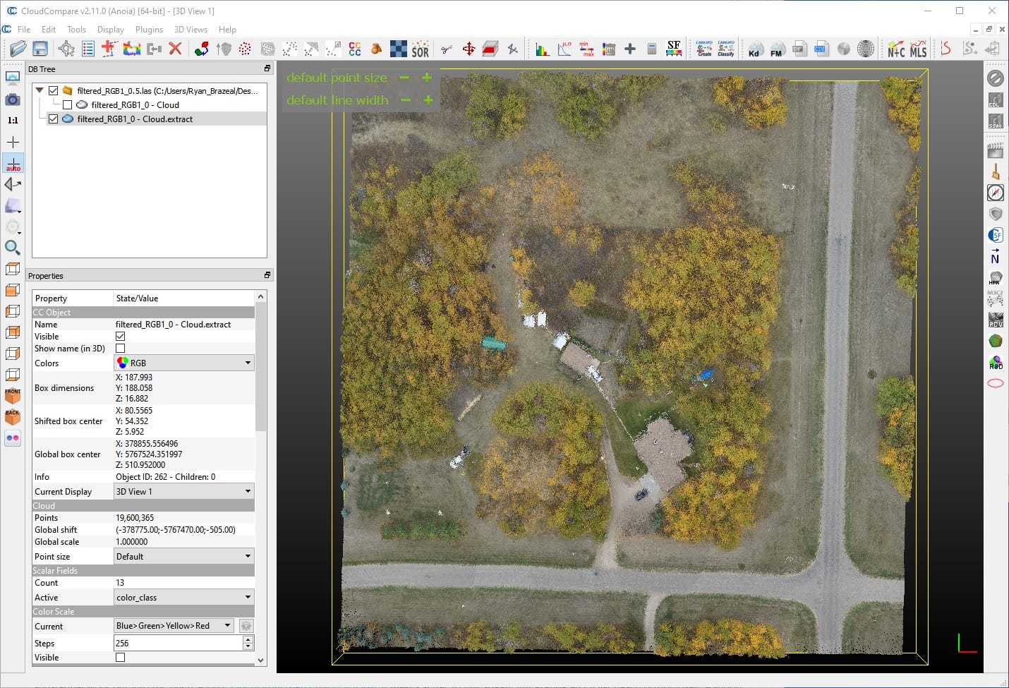
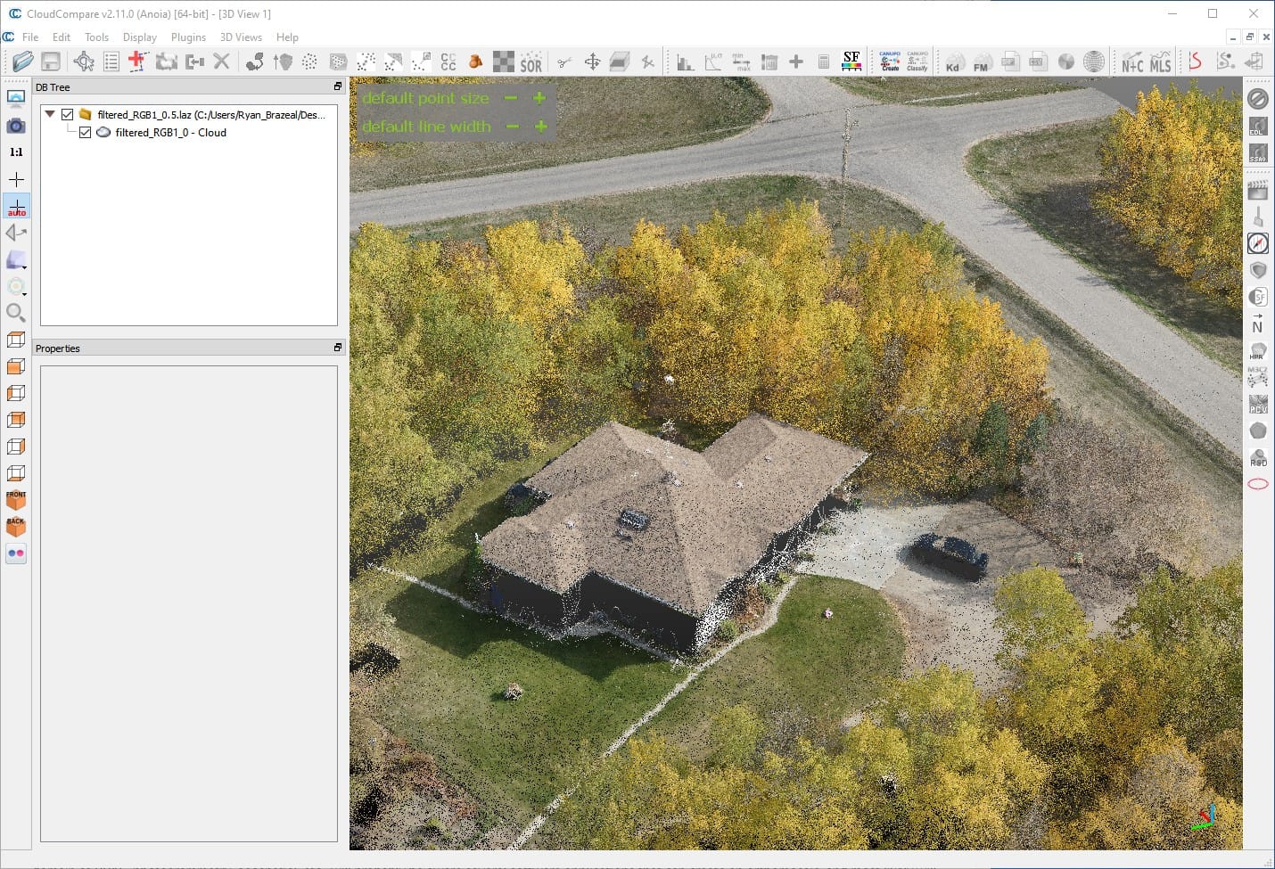
Fig 3.10-9. Colorized point cloud with only colorized points	Fig 3.10-10. Perspective view of the colorized point cloud

---

4. Orthomosaic Generation

Important

A long-term development goal of the OpenMMS Project is to create a rigorous and robust orthomosaic generation application. Given the impressive and substantial work put into the open-source OpenDroneMap Project (ODM), it makes sense to investigate integrating an ODM-based orthomosaic solution within OpenMMS. Don’t hold your breath, but hopefully, this can become a reality someday!

To be thorough, a quick discussion on how to generate an orthomosaic image using OpenMMS collected data is now presented. A user with experience in the domain of RPAS, photogrammetry, geospatial, etc., will probably be aware several software applications that can create an orthomosaic, and most likely will have their own ‘tried-and-true’ favorite solution. This section presents two solutions for generating an orthomosaic image from collected OpenMMS data. The first solution uses only the OpenMMS colorized point cloud and the open-source CloudCompare application. This solution can produce a reasonable medium-resolution orthomosaic geotiff image. The second solution utilizes the previous Pix4Dmapper project, as presented within section 2.9, along with the filtered.las point cloud dataset. The Pix4Dmapper solution enables a high-resolution orthomosaic geotiff image to be quickly produced.

CloudCompare Orthomosaic

Begin by opening the OpenMMS colorized point cloud within CloudCompare. It is recommended to clip the point cloud such that the boundaries of the dataset are straight lines (e.g., rectangular or polygonal shape), see Figure 4-1. Next, with the clipped point cloud dataset selected within the DB Tree list in CloudCompare, from the top menu, select Tools -> Projection -> Rasterize (and contour plot), see Figure 4-2.

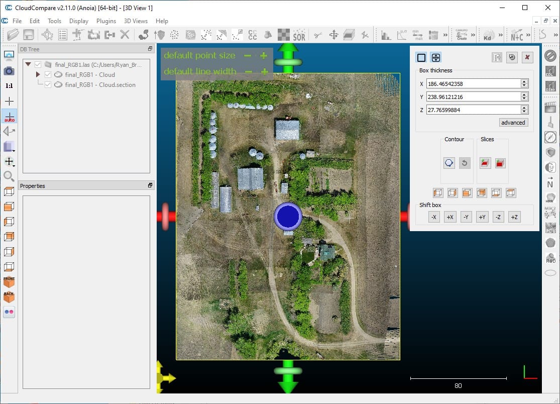
Fig 4-1. Colorized point cloud clipped within CloudCompare

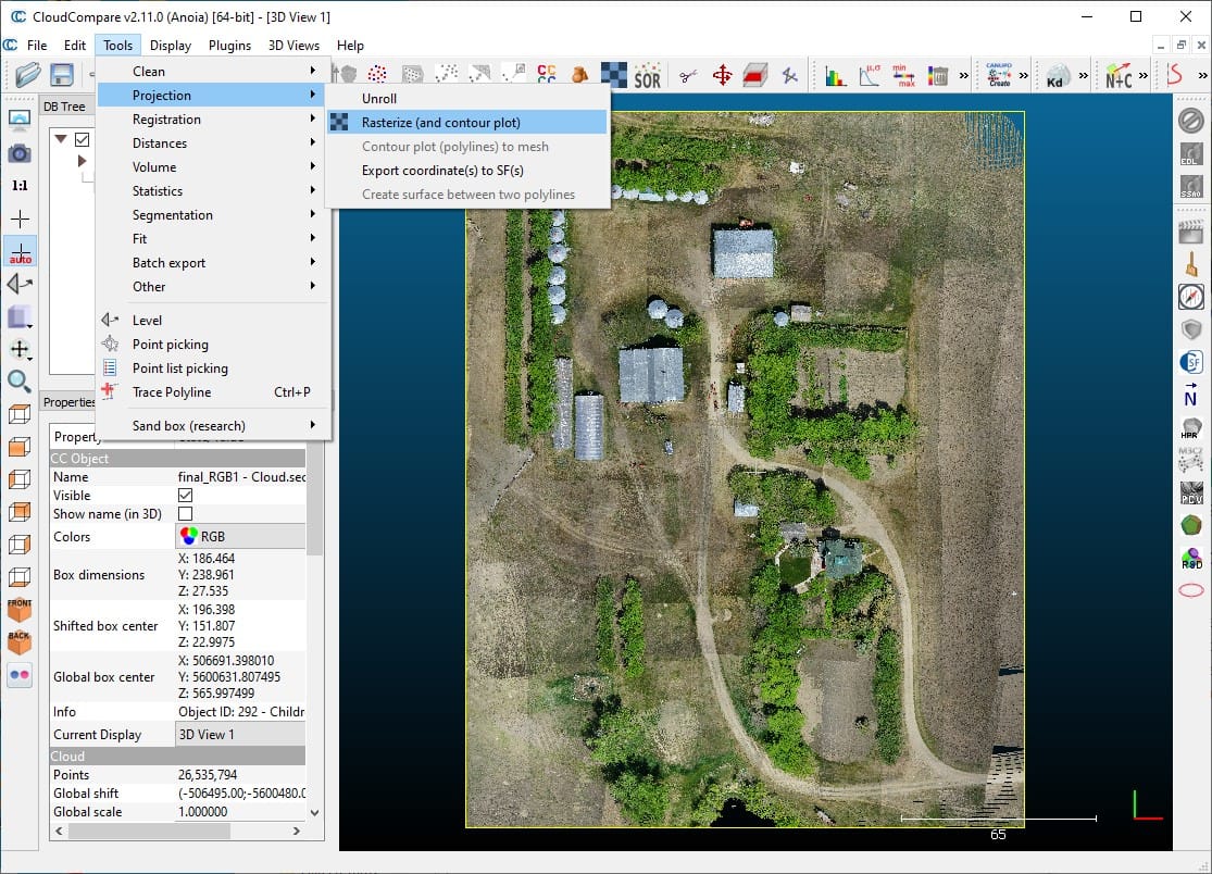
Fig 4-2. Access CloudCompare’s Rasterize features

Next, follow the steps and enter/select the processing options exactly as shown in Figure 4-3. Save the orthomosaic geotiff image to the data collection directory, as shown in Figure 4-4.

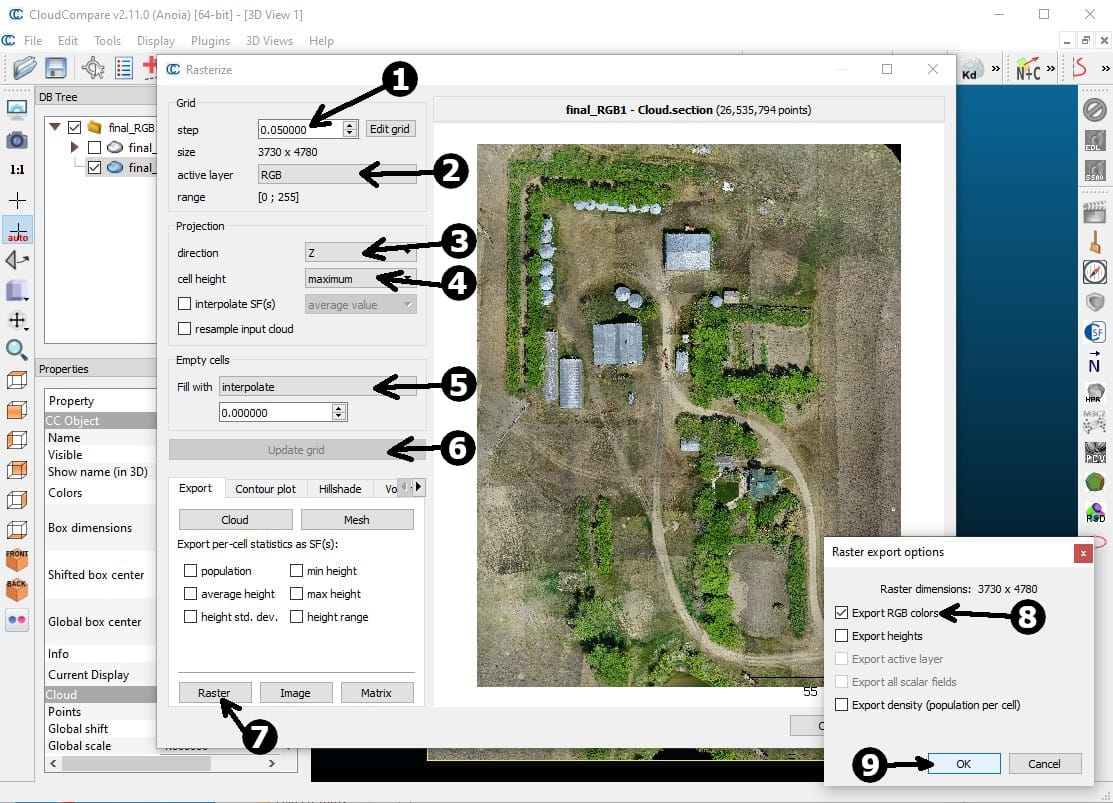
Fig 4-3. Steps and options for generating an orthomosaic in CC

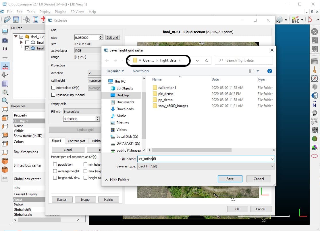
Fig 4-4. Save the orthomosaic to the data collection directory

Pix4Dmapper Orthomosaic

To produce an orthomosaic image using Pix4Dmapper and the data collected from an already calibrated OpenMMS sensor, a slightly modified version of the processing steps as demonstrated within Video 4 of tutorial #1 needs to be performed. Because the sensor is already calibrated, GCPs are not technically required (though using them is always advised) so marking them within the Pix4Dmapper project is unnecessary. The calibration method should also be changed to Accurate Geolocation and Orientation, as shown in Figure 2.9-10. Then, the 1. Initial Processing step needs to be executed.

Open the Processing Options dialog and uncheck the box beside 1. Initial Processing, and check the box beside 3. DSM, Orthomosaic and Index. Set the processing options on the DSM and Orthomosaic tab to those shown in Figure 4-5. From the top menu, click Process -> Import Point Cloud for DSM Generation…, and browse to the data collection directory and select the filtered.las point cloud file. By using the filtered point cloud, the computationally expensive 2. Point Cloud and Mesh processing step within Pix4Dmapper can be bypassed entirely. Lastly, click the Start button in the Processing area on the Pix4Dmapper’s main dialog. Once the orthomosaic processing has finished, a new geotiff image will be available within the Pix4Dmapper project directory –> 3_dsm_ortho subdirectory –> 2_mosaic subdirectory.

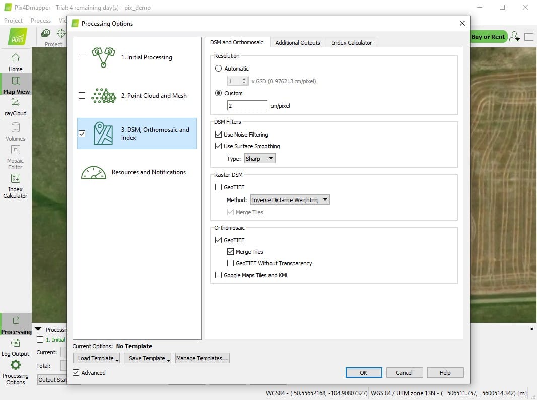
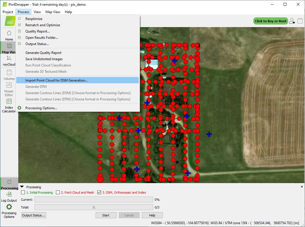
Fig 4-5. Pix4Dmapper Processing Options for orthomosaic creation	Fig 4-6. Import an existing point cloud into Pix4Dmapper
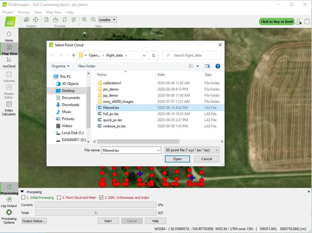
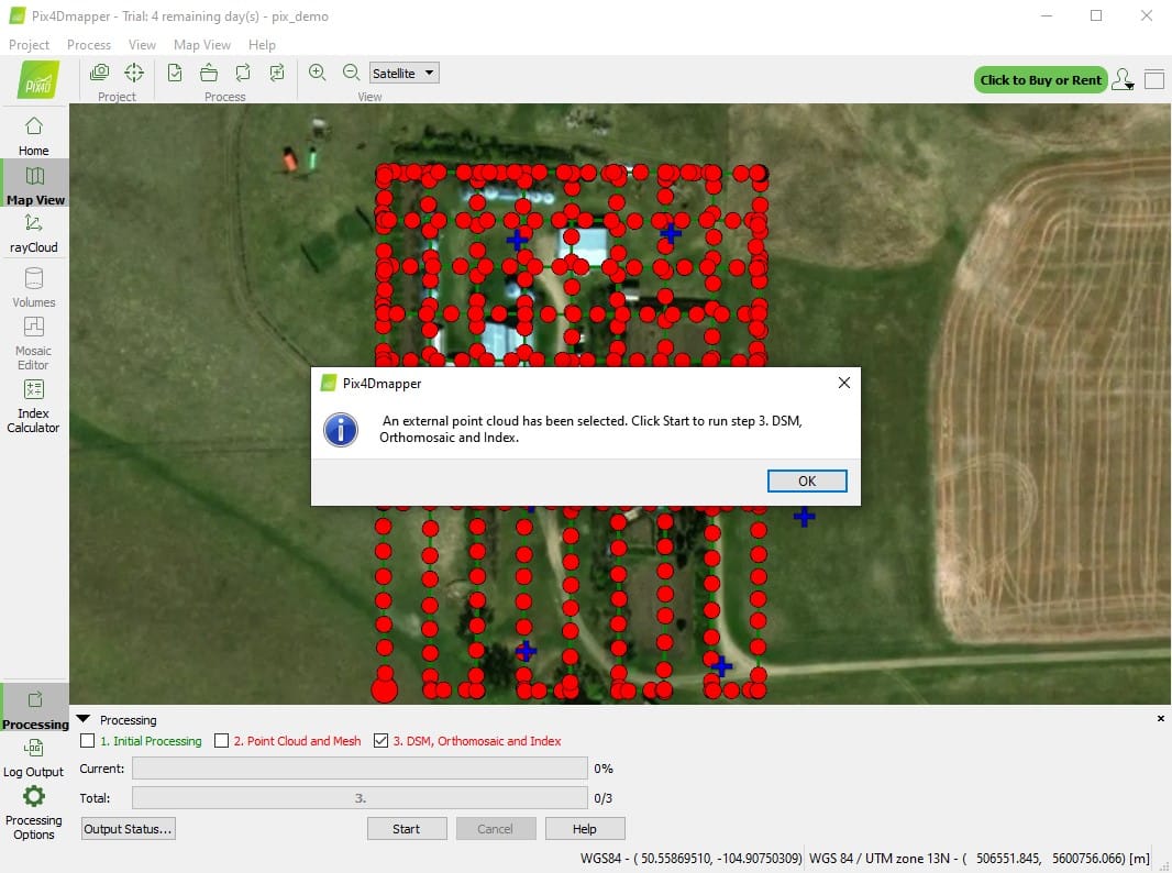
Fig 4-7. Select the OpenMMS filtered lidar point cloud	Fig 4-8. Ready to Start creating the orthomosaic in Pix4Dmapper
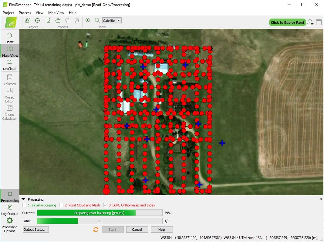
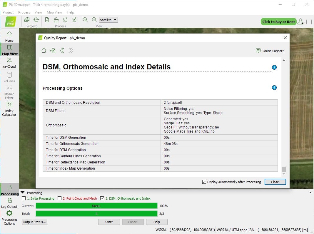
Fig 4-9. Pix4Dmapper orthomosaic progress	Fig 4-10. Orthomosaic produced very quickly

A quick visual comparison of the orthomosaics generated from the two solutions was performed by opening the images within a QGIS Desktop map. The figures below show the orthomosaics (overlaid on a Google Satellite map) as viewed within QGIS.

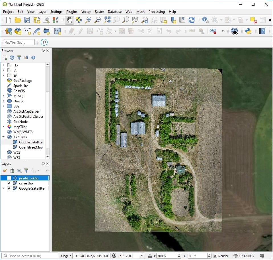
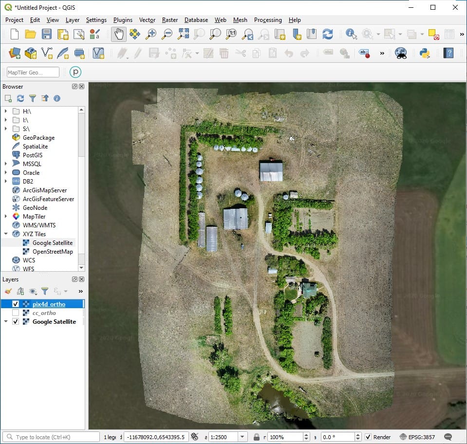
Fig 4-11. CloudCompare orthomosaic 1:2500 scale	Fig 4-12. Pix4Dmapper orthomosaic 1:2500 scale
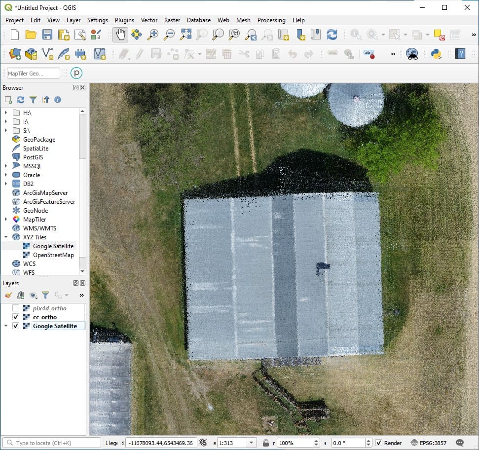
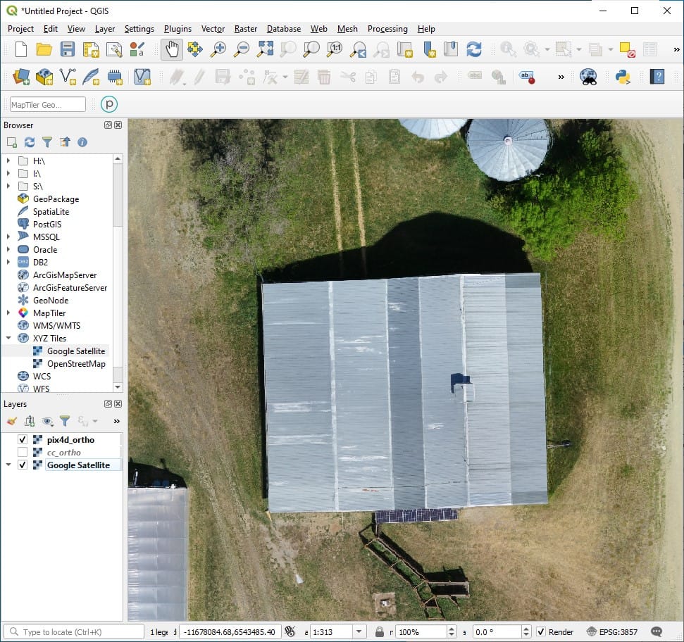
Fig 4-13. CloudCompare orthomosaic 1:300 scale	Fig 4-14. Pix4Dmapper orthomosaic 1:300 scale