OpenMMS Hardware
OpenMMS Open-Source Hardware License
This documentation describes Open Hardware and is licensed under the CERN-OHL-S v2 license.
View the OpenMMS Open-Source Licenses for more details.
CURRENT SENSOR VERSION: 1.3
1. Project Goals
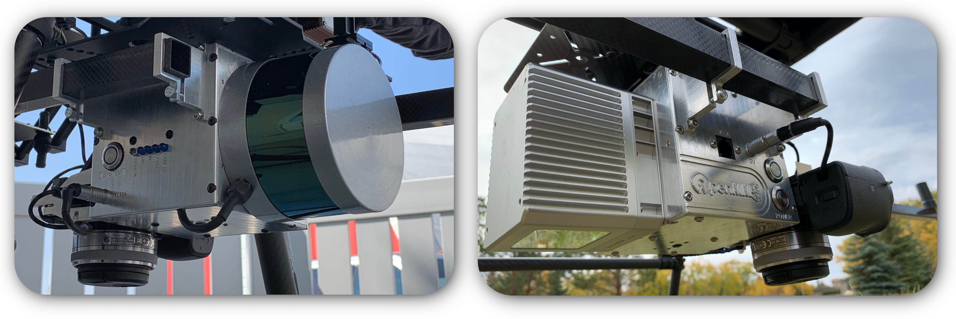
For the OpenMMS Version 1.3 sensor, the primary development goal was to start from a clean slate and completely redesign the sensor. The OpenMMS Version 1.3 sensor project officially began on May the 4th (be with you), 2020. The major goals include:
1. Install and integrate the following components into the system.
2. Design a new aluminum case and new printed circuit boards (PCBs) for:
Minimizing the electrical interference experienced by the onboard IMU sensor on the APX-18 board.
Installing the APX-18 board, so the IMU frame was in a traditional orientation with respect to the vehicle body frame.
Printed circuit board designs that can be created using the Bantam Tools Desktop PCB Milling Machine and are also ready for commercial PCB manufacturing.
Incorporate Lemo power and data ports for connecting to the Sony A6000 camera outside the case.
3. Create simplified software and procedures for calibrating the lever-arm offsets and lidar and camera boresight angles.
4. Create an easy and streamlined data processing and quality assurance post-processing workflow.
2. Specialized Tools
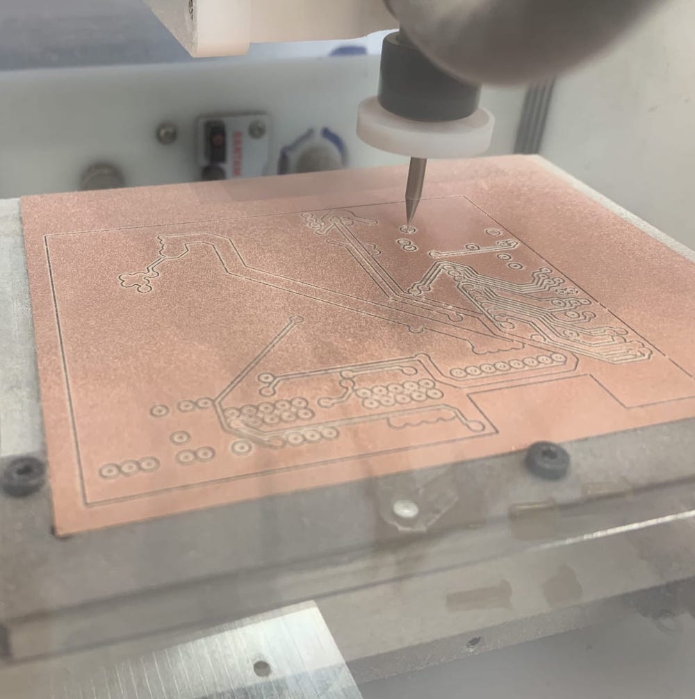
Etching and milling approaches for creating PCBs using desktop manufacturing techniques were investigated. Each method had advantages and disadvantages over the other. Both manufacturing techniques required that the layout (design) of the PCB be completed first. After manufacturing, both methods still needed the vias to be manually connected by soldering. PCB etching was fast and less expensive but required chemical processes and a lot of manual work to complete the circuit board. PCB milling required practically no manual work and produced circuit boards with precise traces. It needed an expensive Computer Numerical Control (CNC) machine, specialized tools, and the knowledge base to convert PCB designs into CNC programs (i.e., manufacturing instructions). In the end, PCB milling was selected because of its ability to produce precise and repeatable results, required little manual work, and allowed open-source hardware files and documentation to be more easily created.
2.1. Bantam Tools Machine
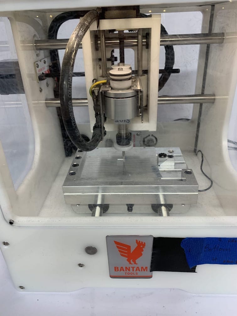
Upon researching the commercially available options for desktop PCB milling machines, the Bantam Tools Desktop PCB Milling Machine was discovered. This machine was capable of milling PCBs, but it was also capable of precisely machining aluminum, dense plastics, and many other materials. Additional benefits of using the Bantam Tools Machine included:
Excellent online documentation, tutorials, and example projects to help get started.
Worked well with Autodesk’s Eagle PCB design and Fusion 360 3D design software.
Easy to learn, machine control software (Bantam Tools Machine Software).
Support for a wide selection of end mills and bits
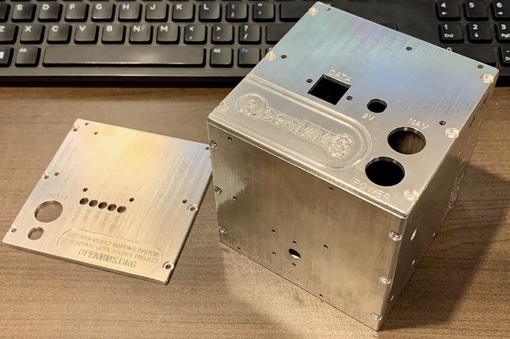
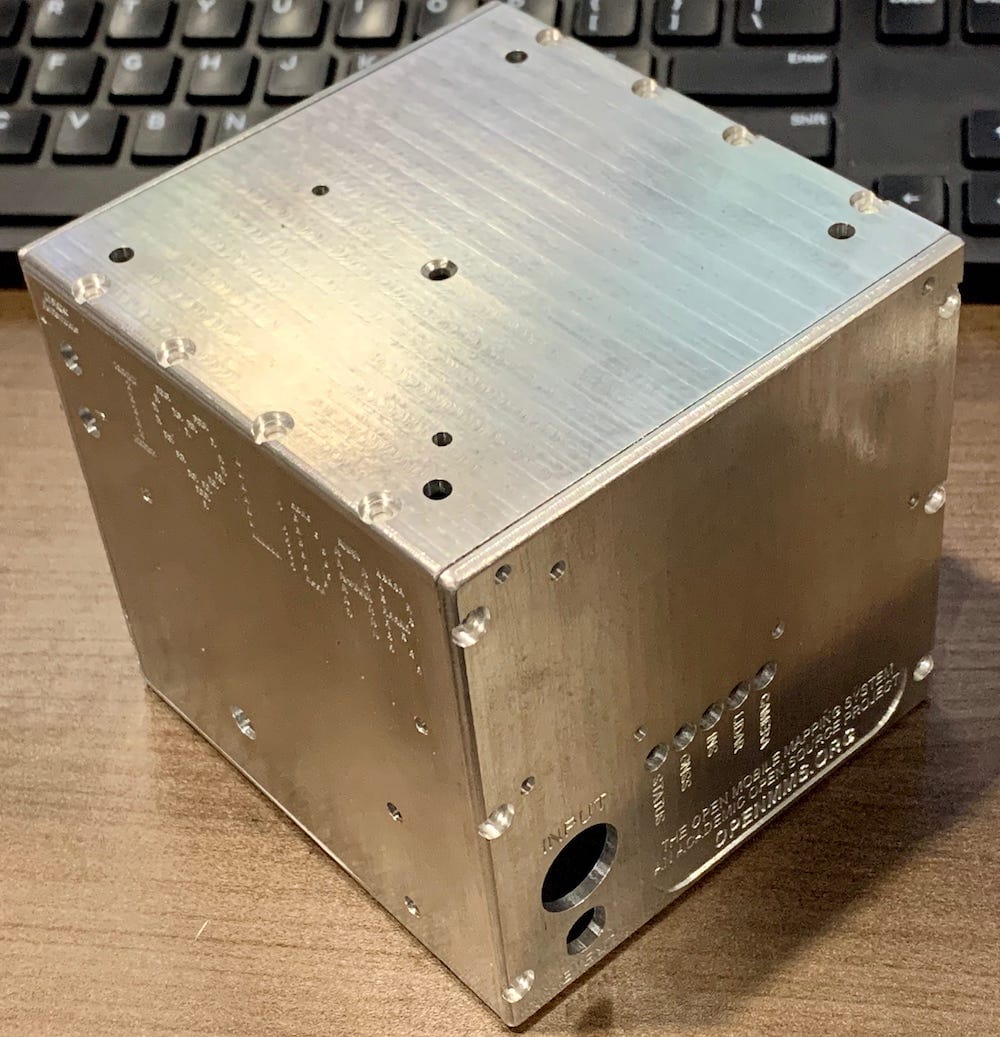
The Bantam Tools Machine did pose a limitation on the size of the machined parts that could be produced. As a result, the aluminum case design utilized six machined main parts, one for each face of the cubed case. The case could then be assembled using metric bolts and Loctite.
2.2. Bantam Tools Machine Setups (BTMS)
There are four different machine setups used during the OpenMMS milling operations using the Bantam Tools Machine.
2.2.1. 1st setup
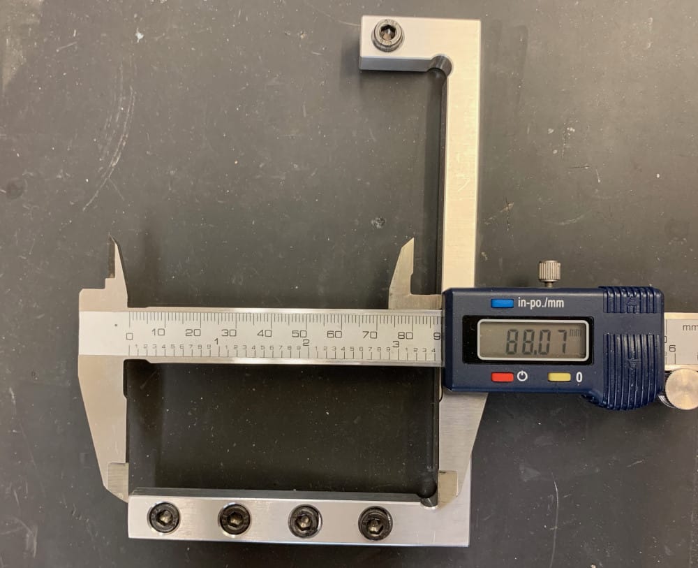
This setup requires the installation of the Precision Fixturing and Toe Clamp Set onto the machine. These instructions explain the installation procedure. However, the left side of the Precision Fixture needs to be shortened, for the aluminum milling operations not to collide with the fixturing. The inside dimension (ID) of the left side of the Precision Fixturing needs to be ~ 88mm. It can easily be shortened using a hacksaw. The images below show the shortened Precision Fixturing installed on the machine.
2.2.2. 2nd setup
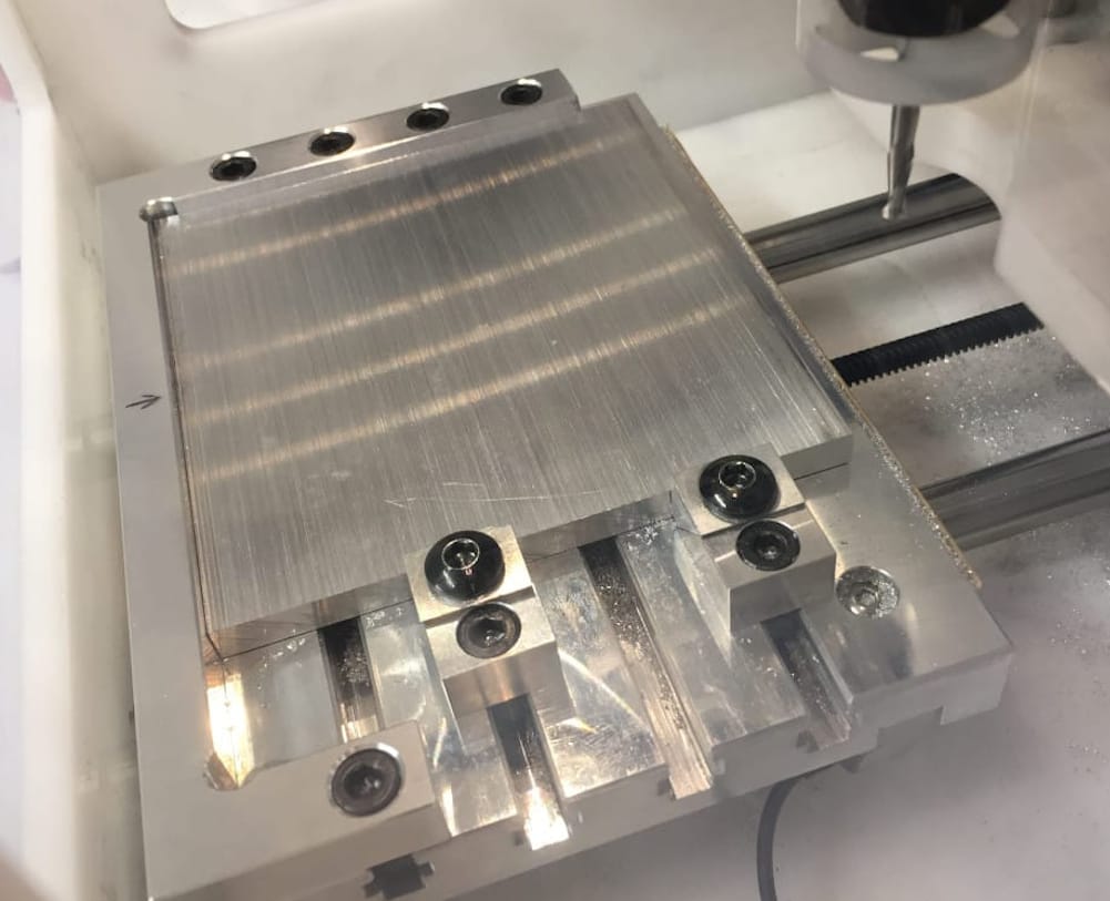
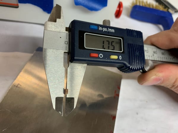
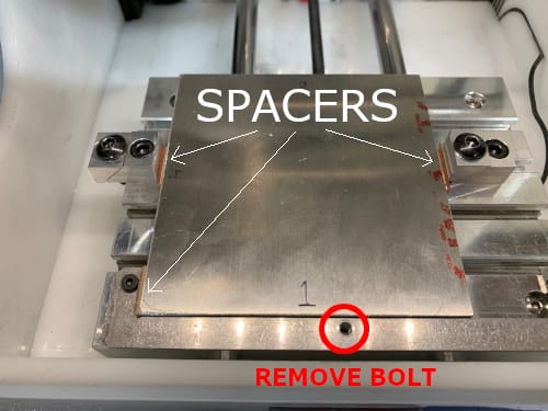
This setup requires the installation of the Alignment Bracket that comes included with the Bantam Tools Machine. However, before the Alignment Bracket is installed, the spoilboard must be removed, which differs from the instructions provided by the manufacturer. Once the Alignment Bracket is installed, the Toe Clamps, from the Precision Fixturing and Toe Clamp Set, are installed on each side of the bracket. To complicate the setup even further, small spacers (of equal dimensions) need to be placed in-between the aluminum material being milled and the clamps on both sides and the left edge of the Alignment Bracket. Using small pieces of PCB blanks works well for this. These spacers allow the End Mill to reach the very edges of the material without colliding with the fixturing. The clamp on the right side is used to secure the material and can be moved around depending on the milled material’s width. The left side clamp is installed backward, and the clamp is positioned rigidly and inline with the small inside left edge of the Alignment Bracket. The final steps are to insert and clamp the aluminum material to be milled, and then remove the middle bolt that secures the Alignment Bracket. Again, this needs to be done to ensure that the End Mill does not collide with this middle bolt. The images below illustrate the small spacers and the installation of the Alignment Bracket for this 2nd setup. A final very important step is to change the Material Placement’s X coordinate setting to the spacer thickness within the Bantam Tools Software. This setting accounts for the installed aluminum material being offset from the Alignment Bracket (i.e., where X = 0.0mm).

2.2.3. 3rd setup
The 3rd setup also requires installing the Alignment Bracket, but now the bracket is installed on top of the spoilboard. The spoilboard needs first to be installed on the machine’s fixed bed, and then the Alignment Bracket is installed. This setup follows the instructions provided by the manufacturer. High-strength, double-sided tape must be used to hold the material to the spoilboard. To easily remove the finished aluminum brackets from the spoilboard, use a small prying tool (e.g., a putty knife) to create a small gap in-between the milled aluminum and the spoilboard. Apply a small amount of 91% isopropyl alcohol into the gap. Gently tilt the entire Bantam Tools Machine to the left and right, as well as forward and backward (being careful not to damage the power cord or USB cord connected to the back of the machine). Tipping the machine allows the alcohol to flow into the double-sided tape and release the part.
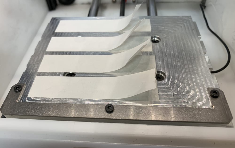
Fig 2.2-6. Alignment Bracket on spoilboard with double-sided tape (3rd setup)
2.2.4. 4th setup
This setup is essentially the same as the 3rd setup, with the only difference being that the Alignment Bracket is not used. High-strength double-sided tape is still required to secure the material to the spoilboard of the machine. The front-left corner of the spoilboard is used as the alignment point for the material. Thus, the precision at which the material is installed on the spoilboard is not very important. Aligning the material on the spoilboard by eye is sufficient. Once again, isopropyl alcohol should be used to release the machined part after the milling operation(s) is complete.
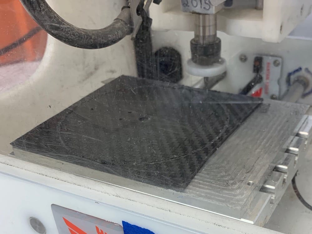
Fig 2.2-7. Carbon fiber plate aligned to the front-left corner of the spoilboard (4th setup)
2.3. Proxxon MICROMOT Tools
Because the case is constructed out of individual aluminum sides, threaded bolt holes need to be machined into the ends (i.e., into the thickness) of the front and back aluminum parts. The Bantam Tools Machine is not capable of performing these end milling tasks. A manual process using a drill press and a hand tap is needed to create these threaded bolt holes. In a continued effort to minimize project costs and only utilize desktop manufacturing techniques, the Proxxon MICROMOT System of Tools was used to complete these machining tasks. The following Proxxon tools were used:
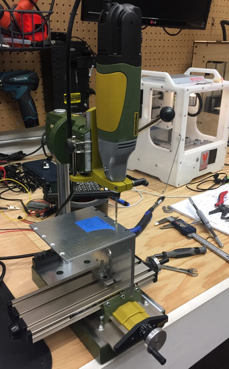
Fig 2.3-1. Proxxon MICROMOT Drill Press
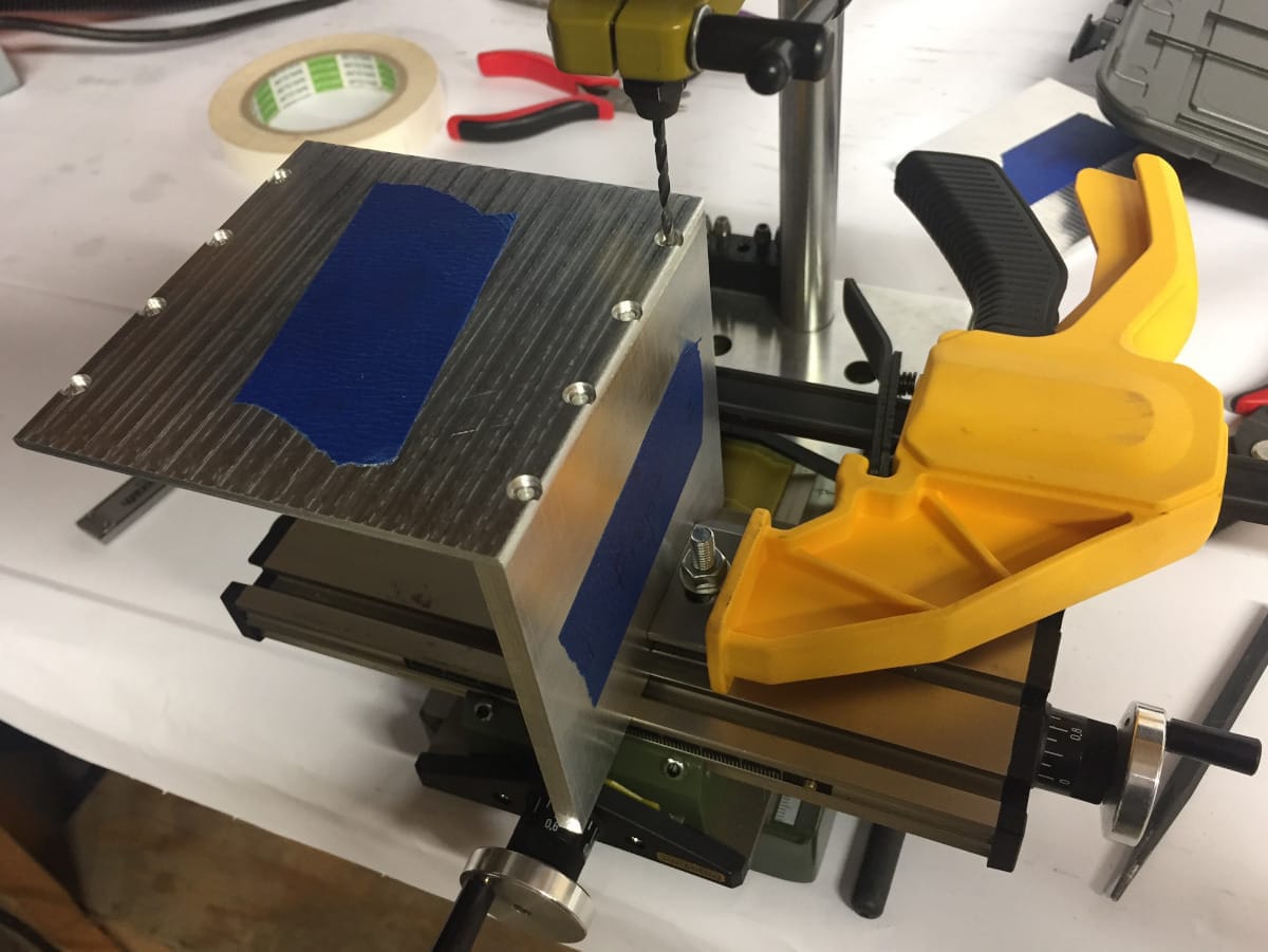
Fig 2.3-2. End milling holes in the front face (top face used as a guide)
Note
The Proxxon Professional Rotary Tool was a little underpowered for the task of drilling the deeper holes in ends of the front and back aluminum pieces. To improve drilling performance, ensure the drill bits being used are sharp, drill small amounts at a time, and try to remove the swarf continuously from the drill hole and the drill bit, using a vacuum and a coarse brush.
3. Getting Started
DISCLAIMER
This documentation provides specific instructions on how the author manufactures and assembles an OpenMMS Version 1.3 sensor. No warranties, of any kind, and no guarantees, of any kind, are included with the following instructions being able to produce an OpenMMS Version 1.3 mobile mapping system.
It is the complete responsibility of the reader of this documentation, to ensure that no personal harm or injuries occur, and no physical damage occurs to any of the individual tools, materials, sensors, components, and electronics, during manufacturing and assembling an OpenMMS Version 1.3 sensor. By continuing to read and execute the following steps; the reader agrees to be responsible for the risks associated with all aspects of the OpenMMS project.
3.1. List of Safety Equipment
|
|
3.2. List of Tools
|
|
3.3. List of Build Materials
|
|
3.4. List of Sensors and Electronics
|
|
3.5. List of Printed Circuit Board Components
NOTE: All components are through-hole (TH)
|
3.6. List of Software
4. Aluminum Parts Manufacturing
4.1. Overview
There are a total of thirteen aluminum parts that need to be manufactured using the Bantam Tools Machine. The Top, Bottom, Left, and Right Faces are machined out of 1/8” thick 6061 aluminum material. All other parts are machined out of 1/4” thick 6061 aluminum material. Pay close attention to the required End Mill for each milling operation and ensure that the Bit Fan is always installed on each End Mill. The Bantam Tools Machine should be cleaned, and swarf removed whenever safely possible. The Fine Dust Collection System or Vacuum Port performance upgrades are highly recommended.
The reader is strongly encouraged to work through the Bantam Tools Fusion 360 Aluminum Rings Getting Started Project before proceeding with manufacturing the OpenMMS aluminum parts. The Getting Started Project provides excellent explanations, does and don’ts, and other valuable information on aluminum milling using the Bantam Tools Machine.
3D Model
Model A: OpenMMS v1.3 Aluminum Case
4.2. Instructions
Each of the thirteen aluminum parts that need to be manufactured is listed below. Notice that the required quantity of each part is listed in the top right corner of each table. The Autodesk Fusion 360 3D design files have been included for each part. If the reader is interested in making edits to these files, the Bantam Tools tool library needs to be set up within their Fusion 360 software. Bantam Tools provides an excellent introduction to setting up and using Fusion 360, an interested reader should view this page. The Bantam Tools Machine instruction files (a.k.a., GCODE files) for all milling operations are included in the correct order of execution. Each GCODE file represents milling operations that use the same tool (i.e., a single End Mill). The order the milling operations are executed is critical!
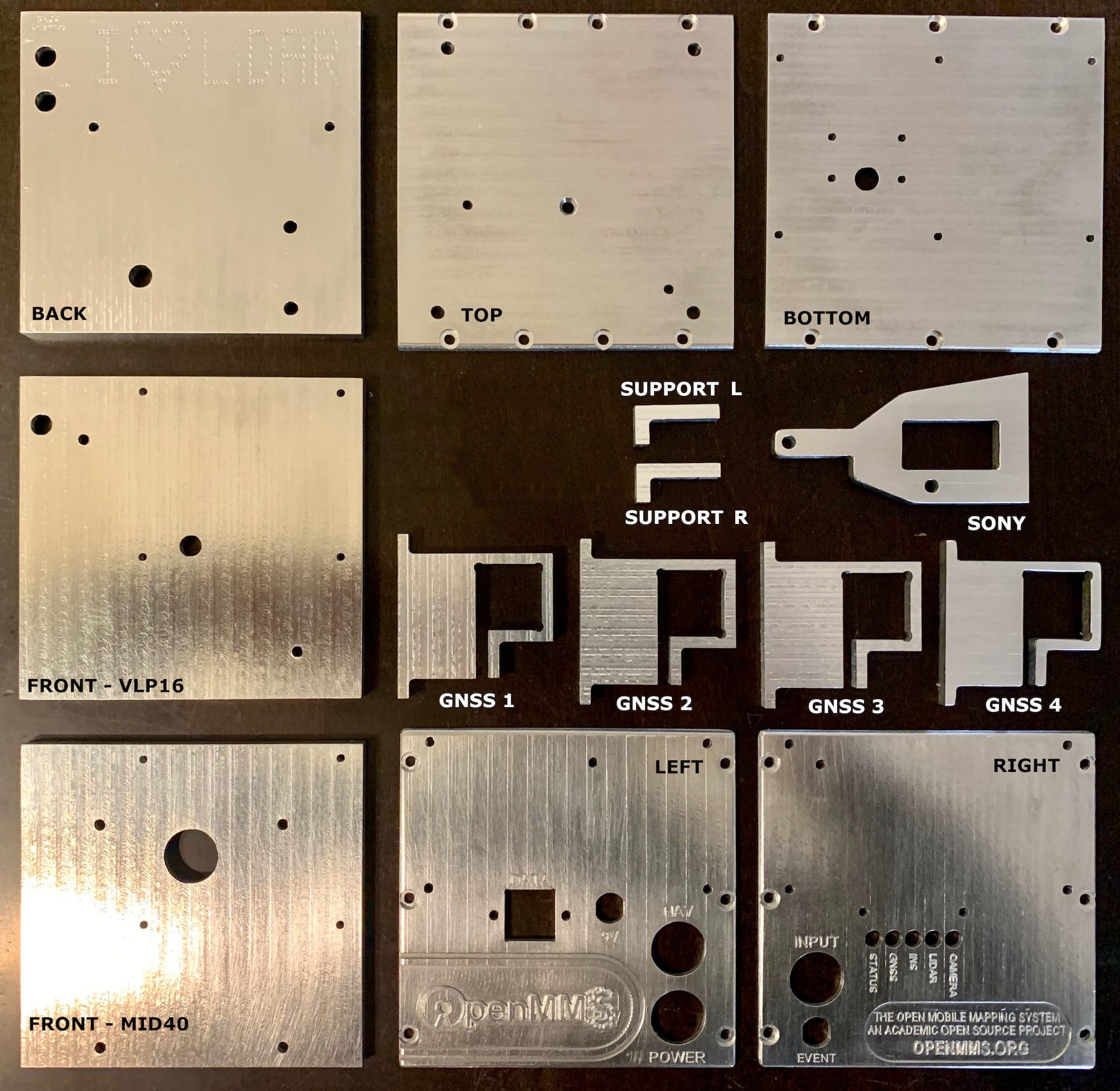
Fig 4.2-1. All thirteen aluminum parts (two front faces are shown, one for each current lidar sensor option)
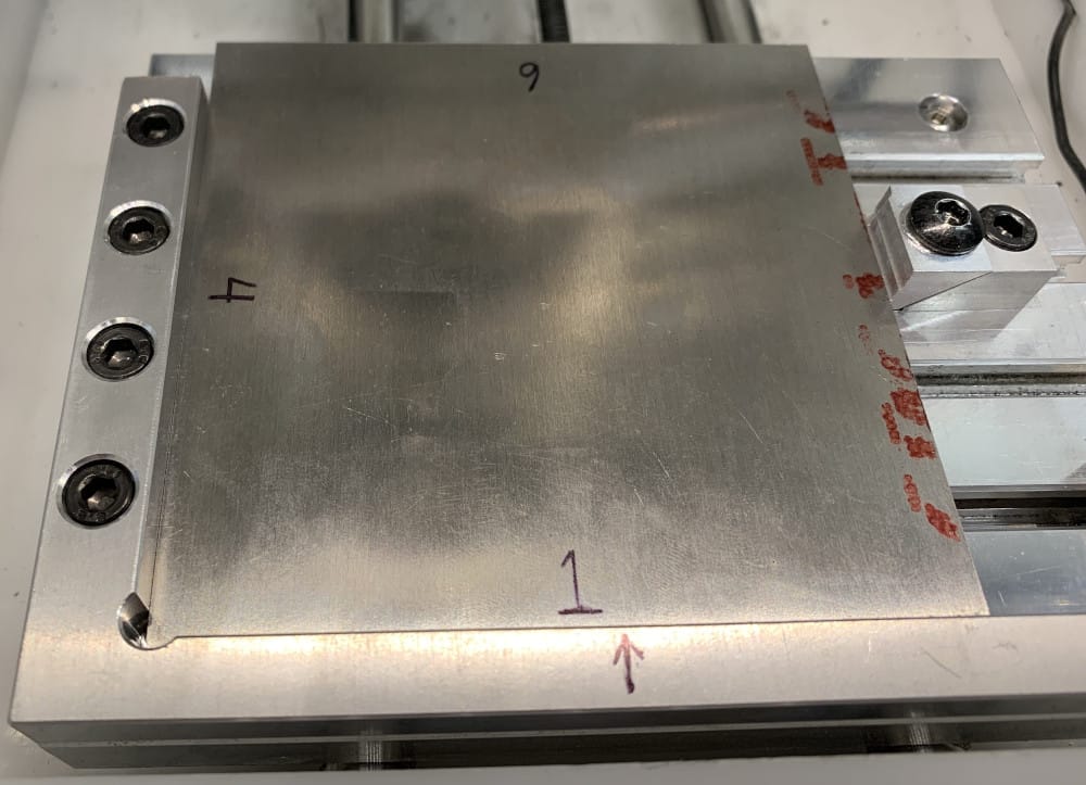
Begin by viewing the edge descriptions image for the part being manufactured and write the number of each listed edge directly on the blank piece of aluminum. The width and height dimensions of the blank are assumed to be the same. Therefore, the orientation of the blanks does not matter. The left and right images show the opposite sides of the same piece of aluminum. The images share the common edge between them, with the piece of aluminum being flipped over like turning the page of a book. For example, the Top Face edge descriptions image illustrates that edge #6 (on side A) and edge #2 (on side B) are the same edges. As the respective milling operations are performed, the written edge numbers will be removed. It is important to keep track of which edge is which throughout the milling operations. It is recommended to either rewrite the edge numbers back onto the aluminum after the milling operation is complete or use pieces of tape with the edge numbers written on them. The tape must be removed before a milling operation is started and replaced after the operation is complete.
Each milling operation requires the aluminum blank to be installed into the Bantam Tools Machine in a particular way. All aluminum milling operations require the aluminum blanks to be installed tight against the left corner of the fixturing bracket. The part tables below, indicate how the aluminum blank must be installed via the Install @ column under the milling operations section. The number listed indicates which edge of the aluminum blank needs to be positioned against the fixturing bracket’s long side (left/right direction). The edge number needs to be facing upwards and, therefore, readable after the aluminum blank is installed in the machine. Figure 4.2-2 illustrates an aluminum blank installed at edge #1.
Attention
If using the efficient approach discussed below, the reader must pay close attention to ensuring the edge numbers for each aluminum blank are maintained throughout the milling operations.
The most efficient approach to milling the aluminum parts is to configure the Bantam Tools Machine using the 1st setup and execute milling operations 1-4 for the respective Face parts and Bracket Blanks, as listed below (totaling eight separate pieces). The milling operations 1-4 will cut the aluminum pieces into the correct X and Y dimensions. Next, configure the Bantam Tools Machine using the 2nd setup and execute milling operations 5-6 on the previous eight respective aluminum pieces. Milling operations 5-6 will plane the aluminum pieces into the correct Z dimensions (i.e., thicknesses). Then, reset the Bantam Tools machine using the 1st setup and execute the remaining milling operations for the six respective Face parts. Lastly, configure the Bantam Tools Machine using the 3rd setup and complete the milling operations for all the Bracket parts, as listed below. An additional benefit to this approach is that after completion of the aluminum parts milling, the Bantam Tools Machine will already be configured into the 3rd setup and therefore, ready to begin with the PCB milling steps.
Danger
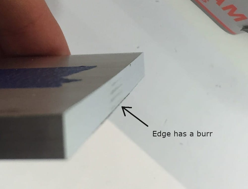
After each milling operation has finished, it is recommended to examine the area(s) on the aluminum that was milled to see if any unwanted material remains (e.g., burr or wire edge). BE CAREFUL WHEN EXAMINING THE PIECE OF ALUMINUM AS A BURR OR WIRE EDGE CAN BE VERY SHARP AND EASILY CUT SKIN. WEARING PROTECTIVE WORK GLOVES WHEN MILLING ALUMINUM IS RECOMMENDED! If a burr or wire edge exists, it can be easily removed using a metal file or possibly even a coarse plastic or brass brush. Figure 4.2-3 illustrates a milled aluminum edge that contains small, but very sharp, burrs.
4.3. Top Face
Table H1: Top Face Design and Manufacturing Files
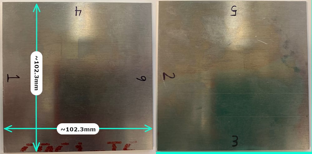
Fig 4.3-1. Top Face - Edge Descriptions
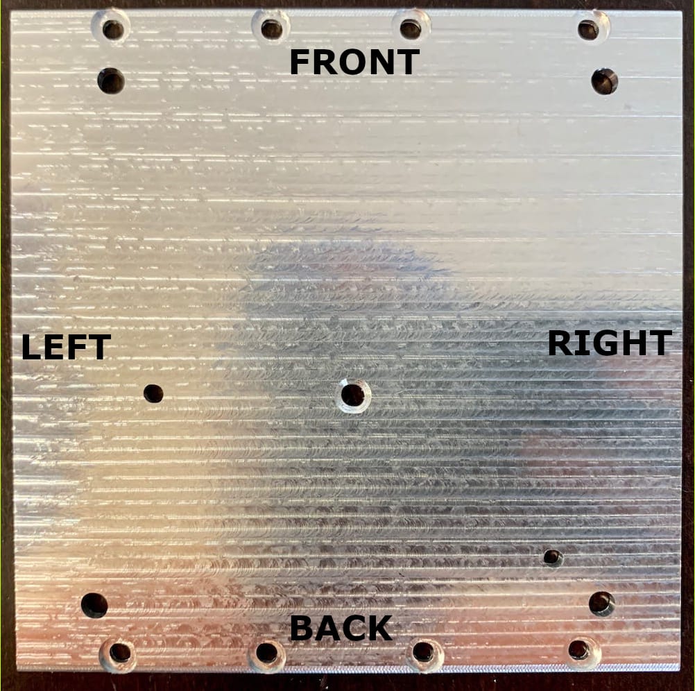
Fig 4.3-2. Completed Top Face
Version: 1.3
Quantity: 1
Material:
1/8” thick 6061 Aluminum
End Mills Required:
Raw Dimensions:
102.3mm x 102.3mm x 3.1mm (approx.)
1/8” Flat End Mill (8F)
1/8” Round End Mill (8R)
1/16” Flat End Mill (16F)
1/16” Round End Mill (16R)
Final Dimensions:
101.0mm x 101.0mm x 2.7mm
Fusion 360 File(s):
MILLING OPERATIONS
Order
Purpose
BTMS
Install @
End Mill
GCODE File:
Bantam Tools Software Configuration
1
2
3
4
5
6
7
8
9
10
11
12
13
14
15
Cut
Cut
Cut
Cut
Plane
Plane
Smooth
Smooth
Holes
Holes
Smooth
Holes
Holes
Notches
Notches
1
1
1
1
2
2
1
1
1
1
1
1
1
1
1
1
2
3
4
1
2
3
5
5
3
5
5
5
1
6
8F
8F
8F
8F
8F
8F
8R
8R
16F
16F
16R
16F
8F
8F
8F
SAME AS PREVIOUS
SAME AS PREVIOUS
4.4. Bottom Face
Table H2: Bottom Face Design and Manufacturing Files

Fig 4.4-1. Bottom Face - Edge Descriptions
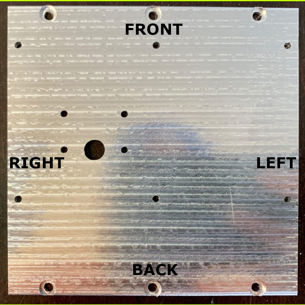
Fig 4.4-2. Completed Bottom Face
Version: 1.3
Quantity: 1
Material:
1/8” thick 6061 Aluminum
End Mills Required:
Raw Dimensions:
102.3mm x 102.3mm x 3.1mm (approx.)
1/8” Flat End Mill (8F)
1/8” Round End Mill (8R)
1/16” Flat End Mill (16F)
Final Dimensions:
101.0mm x 101.0mm x 2.7mm
Fusion 360 File(s):
MILLING OPERATIONS
Order
Purpose
BTMS
Install @
End Mill
GCODE File:
Bantam Tools Software Configuration
1
2
3
4
5
6
7
8
9
10
11
12
Cut
Cut
Cut
Cut
Plane
Plane
Smooth
Smooth
Holes
Holes
Holes
Holes
1
1
1
1
2
2
1
1
1
1
1
1
1
2
3
4
1
2
3
5
5
3
4
4
8F
8F
8F
8F
8F
8F
8R
8R
16F
16F
8F
16F
SAME AS PREVIOUS
SAME AS PREVIOUS
SAME AS PREVIOUS
SAME AS PREVIOUS
4.5. Left Face
Table H3: Left Face Design and Manufacturing Files

Fig 4.5-1. Left Face - Edge Descriptions
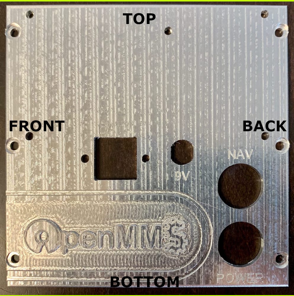
Fig 4.5-2. Completed Left Face
Version: 1.3
Quantity: 1
Material:
1/8” thick 6061 Aluminum
End Mills Required:
Raw Dimensions:
102.3mm x 102.3mm x 3.1mm (approx.)
1/8” Flat End Mill (8F)
1/8” Round End Mill (8R)
1/16” Flat End Mill (16F)
1/32” Flat End Mill (32F)
Metal Engraving Bit (ME)
Final Dimensions:
101.0mm x 101.0mm x 2.7mm
Fusion 360 File(s):
MILLING OPERATIONS
Order
Purpose
BTMS
Install @
End Mill
GCODE File:
Bantam Tools Software Configuration
1
2
3
4
5
6
7
8
9
10
11
12
13
14
15
16
Cut
Cut
Cut
Cut
Plane
Plane
Smooth
Smooth
Smooth
Smooth
Holes
Holes
Holes
Holes
Logo
Engrave
1
1
1
1
2
2
1
1
1
1
1
1
1
1
1
1
1
2
3
4
1
2
2
3
5
6
6
3
3
3
3
3
8F
8F
8F
8F
8F
8F
8R
8R
8R
8R
16F
16F
8F
16F
32F
ME
SAME AS PREVIOUS
SAME AS PREVIOUS
SAME AS PREVIOUS
SAME AS PREVIOUS
SAME AS PREVIOUS
SAME AS PREVIOUS
SAME AS PREVIOUS
SAME AS PREVIOUS
4.6. Right Face
Table H4: Right Face Design and Manufacturing Files

Fig 4.6-1. Right Face - Edge Descriptions
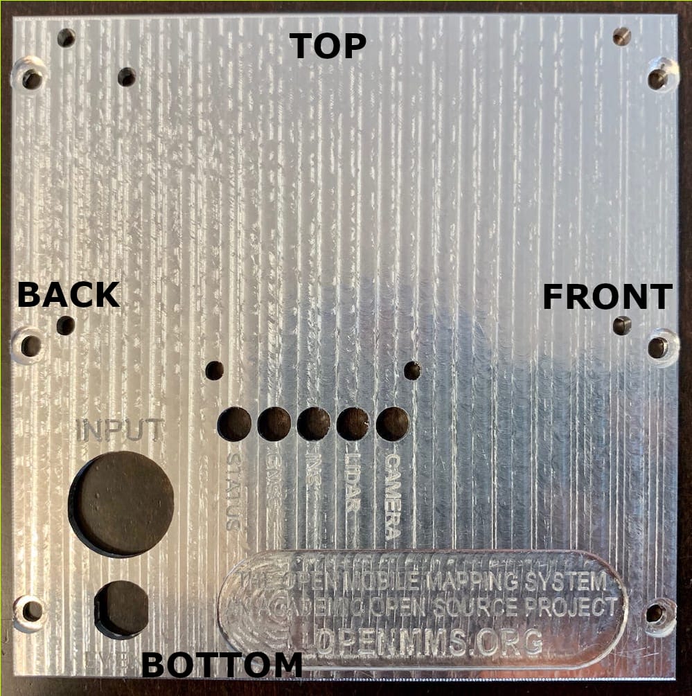
Fig 4.6-2. Completed Right Face
Version: 1.3
Quantity: 1
Material:
1/8” thick 6061 Aluminum
End Mills Required:
Raw Dimensions:
102.3mm x 102.3mm x 3.1mm (approx.)
1/8” Flat End Mill (8F)
1/8” Round End Mill (8R)
1/16” Flat End Mill (16F)
Metal Engraving Bit (ME)
Final Dimensions:
101.0mm x 101.0mm x 2.7mm
Fusion 360 File(s):
MILLING OPERATIONS
Order
Purpose
BTMS
Install @
End Mill
GCODE File:
Bantam Tools Software Configuration
1
2
3
4
5
6
7
8
9
10
11
12
13
14
15
Cut
Cut
Cut
Cut
Plane
Plane
Smooth
Smooth
Smooth
Smooth
Holes
Holes
Holes
Holes
Engrave
1
1
1
1
2
2
1
1
1
1
1
1
1
1
1
1
2
3
4
1
2
2
3
5
6
6
3
3
3
3
8F
8F
8F
8F
8F
8F
8R
8R
8R
8R
16F
16F
16F
8F
ME
SAME AS PREVIOUS
SAME AS PREVIOUS
SAME AS PREVIOUS
SAME AS PREVIOUS
SAME AS PREVIOUS
SAME AS PREVIOUS
SAME AS PREVIOUS
SAME AS PREVIOUS
4.7. Front Face
Table H5: Front Face Design and Manufacturing Files

Fig 4.7-1. Front Face - Edge Descriptions
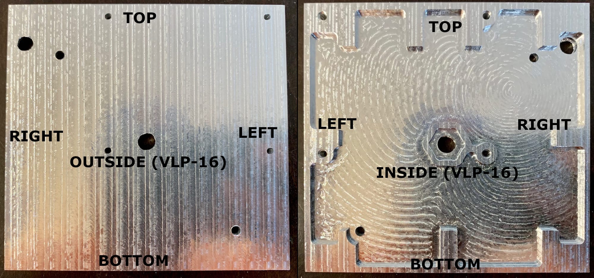
Fig 4.7-2. Completed Front Face (VLP-16) *
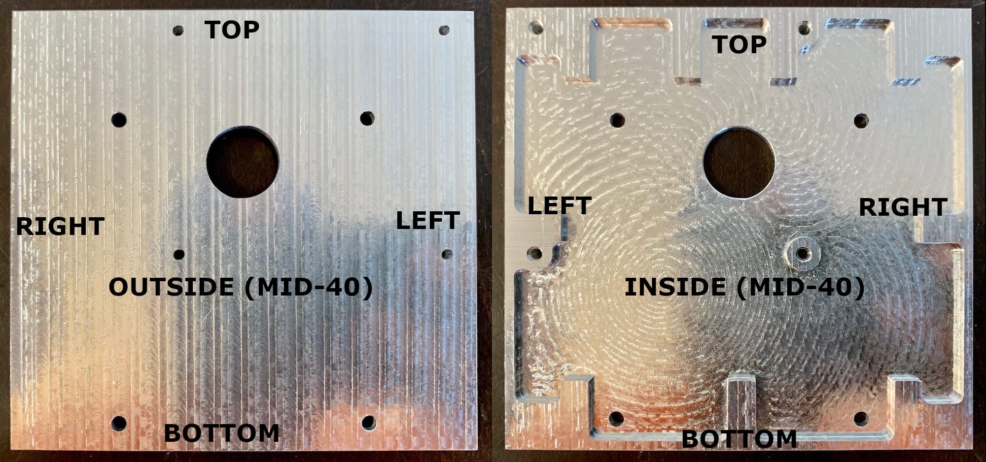
Fig 4.7-3. Completed Front Face (MID-40) **
Version: 1.3
Quantity: 1
Material:
1/4” thick 6061 Aluminum
End Mills Required:
Raw Dimensions:
102.3mm x 102.3mm x 6.4mm (approx.)
1/8” Flat End Mill (8F)
1/16” Flat End Mill (16F)
Final Dimensions:
101.0mm x 95.6mm x 5.8mm
Fusion 360 File(s):
MILLING OPERATIONS
Order
Purpose
BTMS
Install @
End Mill
GCODE File:
Bantam Tools Software Configuration
1
2
3
4
5
6
7*
8*
7**
8**
9
Cut
Cut
Cut
Cut
Plane
Plane
Holes
Holes
Holes
Holes
Holes
1
1
1
1
2
2
1
1
1
1
1
1
2
3
4
4
3
4
4
4
4
4
8F
8F
8F
8F
8F
8F
8F
8F
8F
8F
16F
4.8. Back Face
Table H6: Back Face Design and Manufacturing Files
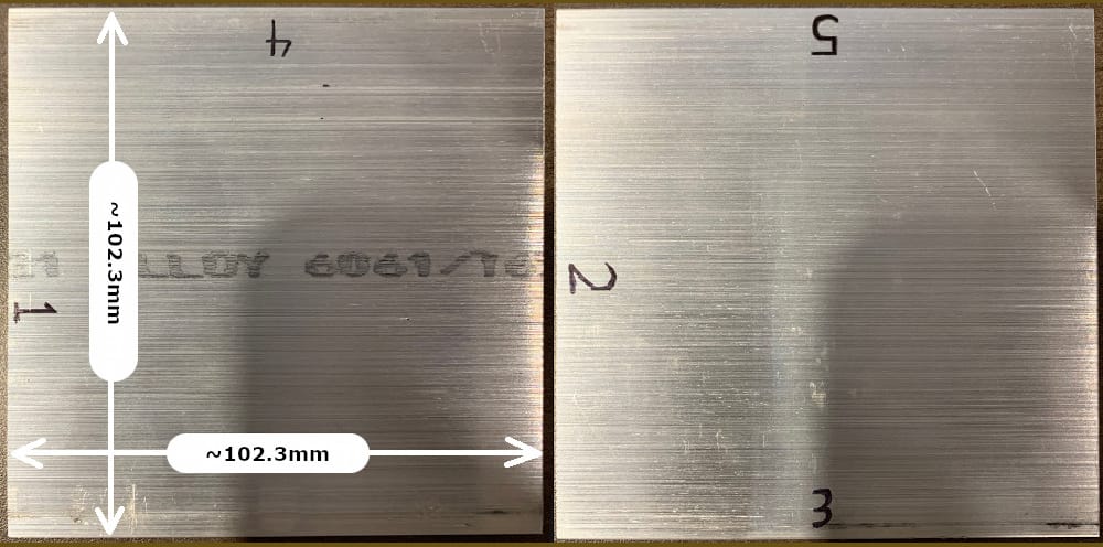
Fig 4.8-1. Back Face - Edge Descriptions
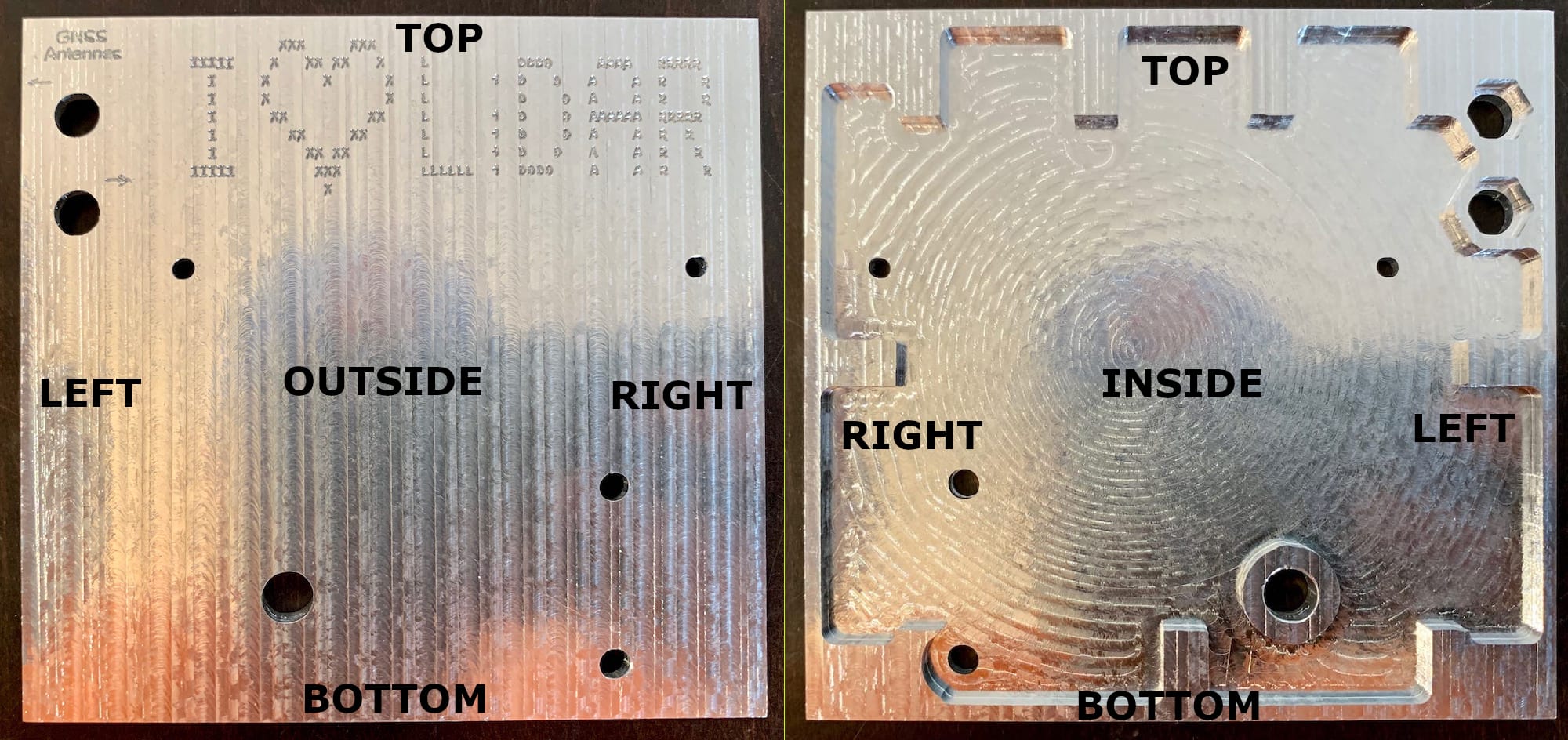
Fig 4.8-2. Completed Back Face
Version: 1.3
Quantity: 1
Material:
1/4” thick 6061 Aluminum
End Mills Required:
Raw Dimensions:
102.3mm x 102.3mm x 6.4mm (approx.)
1/8” Flat End Mill (8F)
1/16” Flat End Mill (16F)
Metal Engraving Bit (ME)
Final Dimensions:
101.0mm x 95.6mm x 5.8mm
Fusion 360 File(s):
MILLING OPERATIONS
Order
Purpose
BTMS
Install @
End Mill
GCODE File:
Bantam Tools Software Configuration
1
2
3
4
5
6
7
8
9
10
Cut
Cut
Cut
Cut
Plane
Plane
Holes
Holes
Holes
Engrave
1
1
1
1
2
2
1
1
1
1
1
2
3
4
4
3
4
4
4
5
8F
8F
8F
8F
8F
8F
8F
8F
16F
ME
4.9. Bracket Blanks
The remaining seven aluminum parts (all a type of support bracket) are manufactured out of 1/4” thick 6061 aluminum. An additional TWO aluminum blanks milled so they have the same final dimensions as the front and back parts, are needed to have enough aluminum material to mill the support brackets.
On the 1st bracket blank, the Sony bracket, both reinforcement brackets, and the first of the four GNSS brackets can be milled. Here is the brackets layout for the 1st blank. On the 2nd bracket blank, the remaining three GNSS brackets can be milled; here is the brackets layout for the 2nd blank.
Table H7: Bracket Blank Design and Manufacturing Files
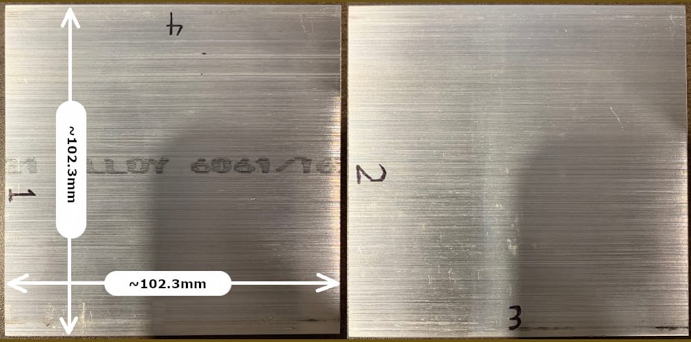
Fig 4.9-1. Bracket Blank - Edge Descriptions
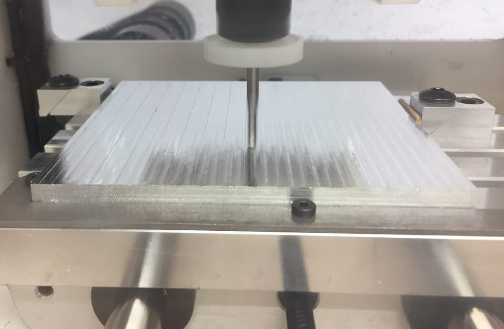
Fig 4.9-2. Completed Bracket Blank
Version: 1.3
Quantity: 2
Material:
1/4” thick 6061 Aluminum
End Mills Required:
Raw Dimensions:
102.3mm x 102.3mm x 6.4mm (approx.)
1/8” Flat End Mill (8F)
Final Dimensions:
101.0mm x 101.0mm x 5.8mm
Fusion 360 File(s):
MILLING OPERATIONS
Order
Purpose
BTMS
Install @
End Mill
GCODE Files:
Bantam Tools Software Configurations
1
2
3
4
5
6
Cut
Cut
Cut
Cut
Plane
Plane
1
1
1
1
2
2
1
2
3
4
4
3
8F
8F
8F
8F
8F
8F
4.10. Sony Bracket
Table H8: Sony Bracket Design and Manufacturing Files
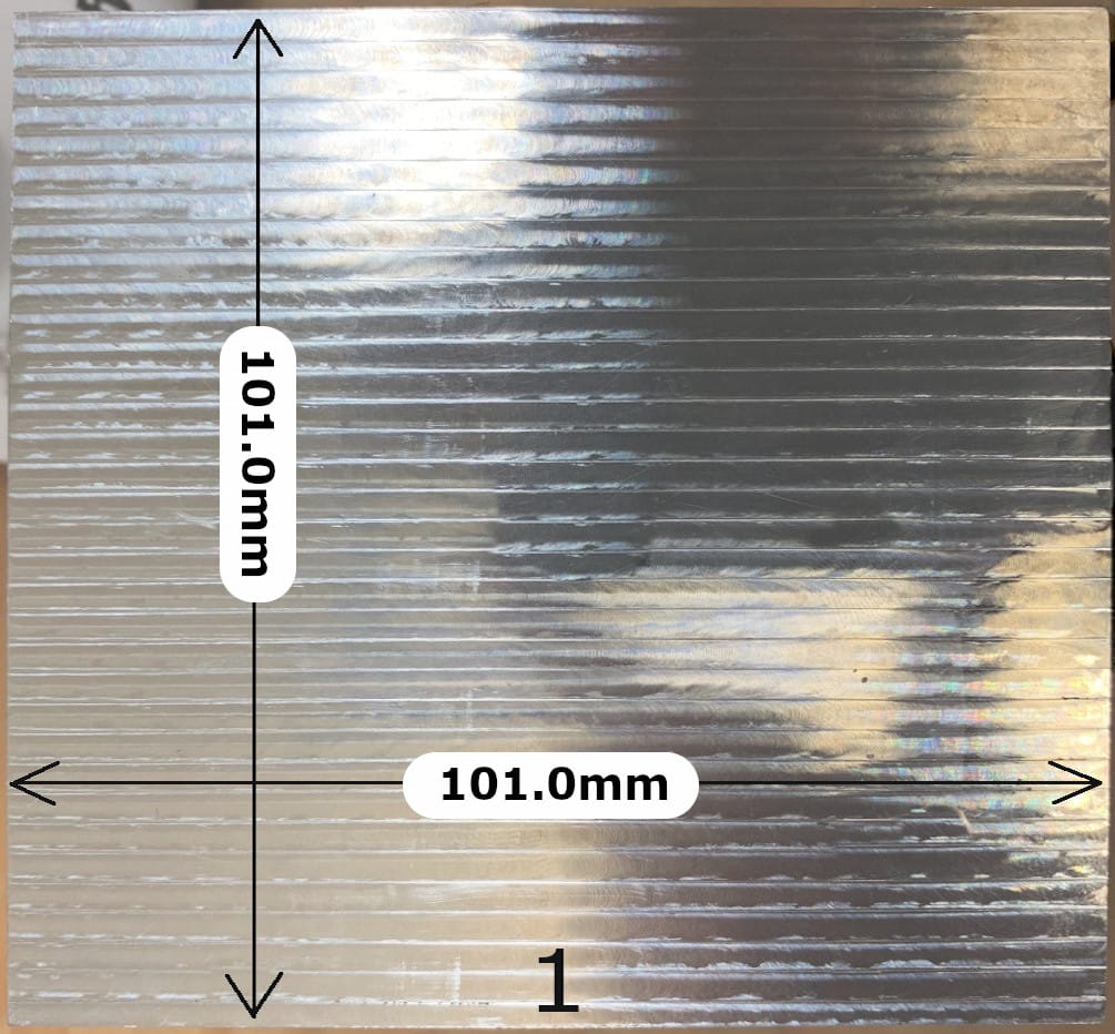
Fig 4.10-1. 1/4” Blank - Edge Descriptions
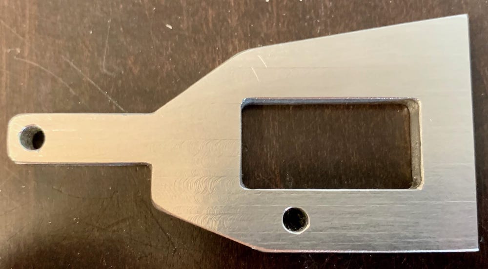
Fig 4.10-2. Completed Sony Bracket
Version: 1.3
Quantity: 1
Material:
1/4” thick 6061 Aluminum
End Mills Required:
Blank Dimensions:
101.0mm x 101.0mm x 5.8mm
1/8” Flat End Mill (8F)
Fusion 360 File(s):
MILLING OPERATIONS
Order
Purpose
BTMS
Install @
End Mill
GCODE Files:
Bantam Tools Software Configurations
1
Cut
3
1 on Blank 1
8F
4.11. Reinforcing Bracket
Table H9: Reinforcing Bracket Design and Manufacturing Files
Fig 4.11-1. 1/4” Blank - Edge Descriptions
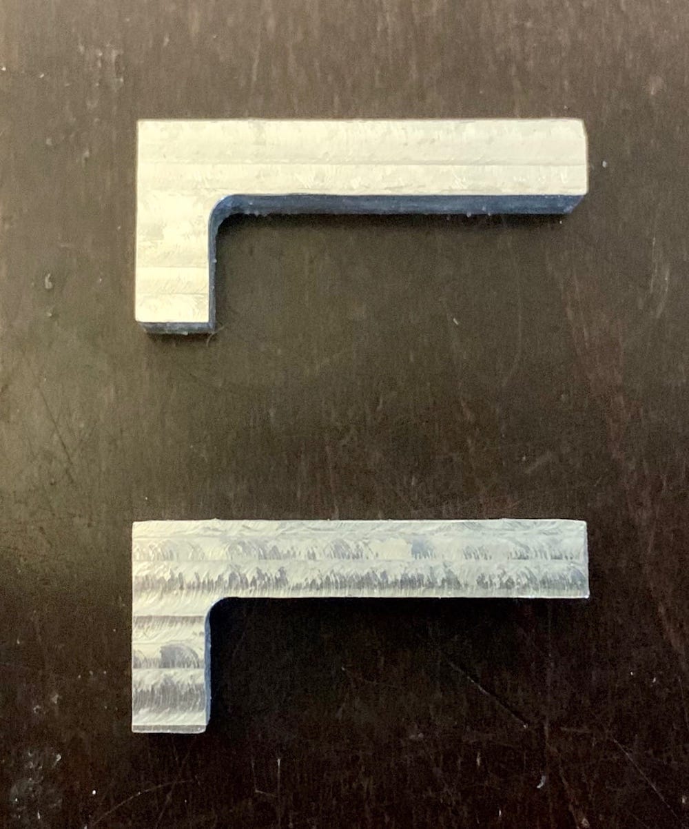
Fig 4-11.2. Completed Reinforcing Brackets
Version: 1.3
Quantity: 2
Material:
1/4” thick 6061 Aluminum
End Mills Required:
Blank Dimensions:
101.0mm x 101.0mm x 5.8mm
1/8” Flat End Mill (8F)
Fusion 360 File(s):
See Sony_Bracket_Design.zip
MILLING OPERATIONS
Order
Purpose
BTMS
Install @
End Mill
GCODE Files:
Bantam Tools Software Configurations
1
2
Cut
Cut
3
3
1 on Blank 1
1 on Blank 1
8F
8F
4.12. GNSS Antenna Bracket
Attention
Pay close attention to the information displayed in the Bantam Tools Software Configurations image for each of the GNSS brackets. Each bracket is positioned on the respective 1/4” aluminum bracket blank to optimize the usable aluminum. The position of each GNSS bracket on the aluminum blanks is defined by the Placement settings for each GCODE file in the Bantam Tools Machine Software (not to be confused with the Material Placement settings).
Table H10: GNSS Antenna Bracket Design and Manufacturing Files
Fig 4.12-1. 1/4” Blank - Edge Descriptions
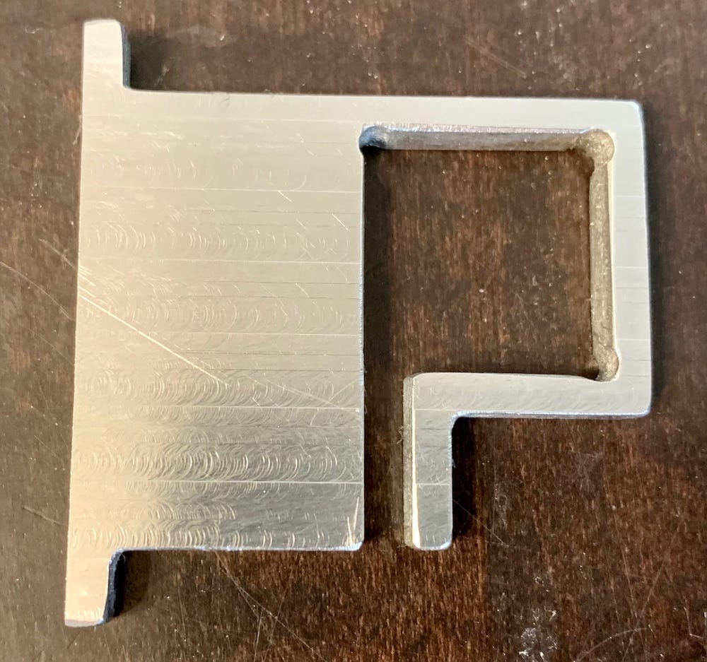
Fig 4-12.2. Completed GNSS Bracket
Version: 1.3
Quantity: 4
Material:
1/4” thick 6061 Aluminum
End Mills Required:
Blank Dimensions:
101.0mm x 101.0mm x 5.8mm (x2)
1/8” Flat End Mill (8F)
Fusion 360 File(s):
MILLING OPERATIONS
Order
Purpose
BTMS
Install @
End Mill
GCODE Files:
Bantam Tools Software Configurations
1
2
3
4
Cut
Cut
Cut
Cut
3
3
3
3
1 on Blank 1
1 on Blank 2
1 on Blank 2
1 on Blank 2
8F
8F
8F
8F
SAME AS PREVIOUS
SAME AS PREVIOUS
4.13. After Milling
It is recommended to use a metal file to gently round/break the sharp 90 degree edges of the manufactured parts after being milled by the Bantam Tools Machine. During assembly, many tight-fitting connections need to be made within the case. By having ‘softer’ aluminum edges, your hands will thank you. It is also recommended to scour all surfaces of the manufactured parts thoroughly. Scotch-Brite abrasive pads or a softer metal brush (e.g., brass) work well for this task. The goal is to remove any tiny aluminum debris/swarf from the manufactured parts. These small pieces of aluminum could cause electrical damage (i.e., create short-circuits) on the sensitive (and costly) sensors and components inside the case. Additional cleaning and finishing steps will be performed at a later stage in the manufacturing process. One last (subjective) benefit to scouring the aluminum parts is, the machining marks on the aluminum surfaces, created by the end mills, can largely be removed. As a result, the aluminum parts will have a ‘nicer’ appearance.
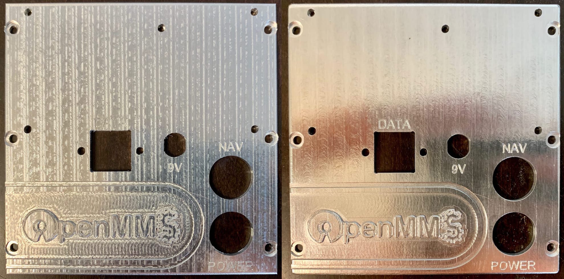
Fig 4.13-1. Left face before (left image) and after (right image) scouring
4.14. Test Fit the Case
With all the aluminum parts now manufactured, the next step is to test fit the six faces of the case together. Cut thin strips of the high-strength double-sided Nitto tape and apply them to all four edge surfaces of the front and back aluminum parts. Next, align and stick the top face to the front and back faces, followed by attaching the bottom face to the front and back faces. Use the labels in the previous parts’ images to figure out how the six faces correctly go together.
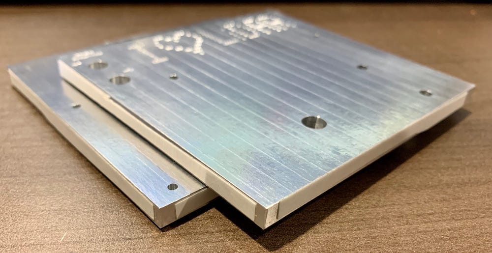
Fig 4.14-1. Nitto tape on front and back faces’ edge surfaces
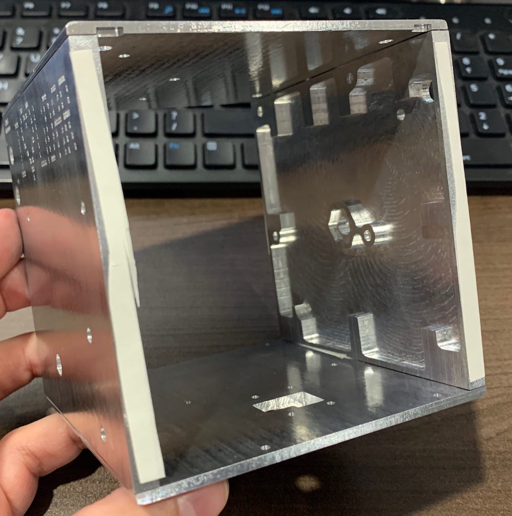
Fig 4.14-2. Top and bottom stuck to front and back
Lastly, stick the left and right faces to the front and back faces. You should see some small gaps between the faces due to the thickness of the Nitto tape. The left and right faces may seem slightly short from top to bottom (again, this is due to the thickness of the tape). Check for any apparent errors in each of the six faces. If needed, fix/re-manufacture any of the faces now, before proceeding.
4.15. Drilling and Tapping Holes
“SLOW AND STEADY IS THE NAME OF THE GAME!!!”
4.15.1. Case Holes
This step is the most labor-intensive part of the entire OpenMMS project! While the case is securely held together by the Nitto tape (double-check that the six case faces are exactly aligned), install the entire case on the Proxxon Compound Table underneath the Proxxon Rotary Tool (i.e., drill press). A quick clamp with the rubber pads removed works well to secure the case to the compound table. Be careful when the clamp ends are compressing the front and back faces as only the Nitto tape is securing these faces to the top, bottom, and sides. Install a 3/32” drill bit into the Rotary Tool. Adjust the drill stand, so the end of the drill bit is a few millimeters above the case. Using the adjustment dials on the compound table, precisely align the drill bit (front to back and left to right) with the first hole to be drilled. As previously mentioned, it helps to use a new, sharp drill bit when machining these holes and remove the aluminum swarf from the drill bit and from inside the hole as often as possible. It is recommended to drill entirely through the thicker aluminum sections on the front and back faces, creating a drilled ‘tunnel’ from the outside edges to the inside of the front and back faces. By doing this, the tapping process (i.e., creating threads inside the holes) is easier, as the aluminum swarf created by the tap has a means of leaving the tunnel.

Fig 4.15-1. Case under the Proxxon ‘drill press’
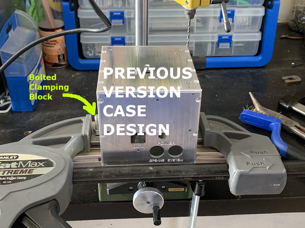
Fig 4.15-2. Quick clamp installing case on the compound table
Start the drilling process by drilling the eight holes for the top face of the case. The holes need to be ~ 15mm in depth to go all the way through the thicker sections of the front and back faces. The Proxxon drill stand has a depth gauge that can be used to quickly and easily see the current drilled hole’s depth. With the Rotary tool off, plunge the drill bit until it touches the aluminum (where drilling would begin). Manually observe the depth gauge’s number. Subtracting the desired depth from this number will indicate the gauge number when the currently drilled hole’s depth has been achieved. Be careful when approaching the desired depth, as the drill bit may become jammed and potentially break.
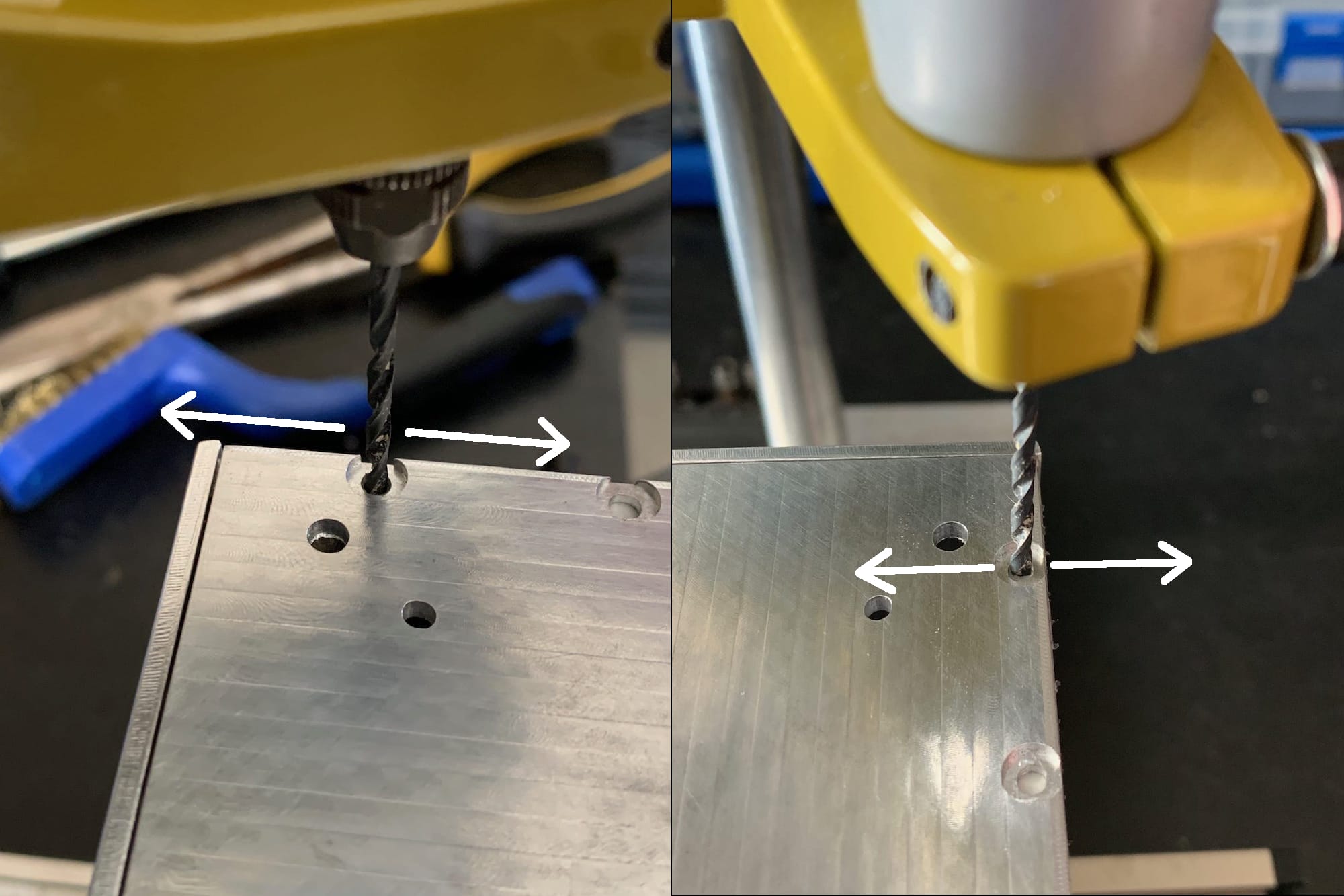
Fig 4.15-3. Align front to back and left to right
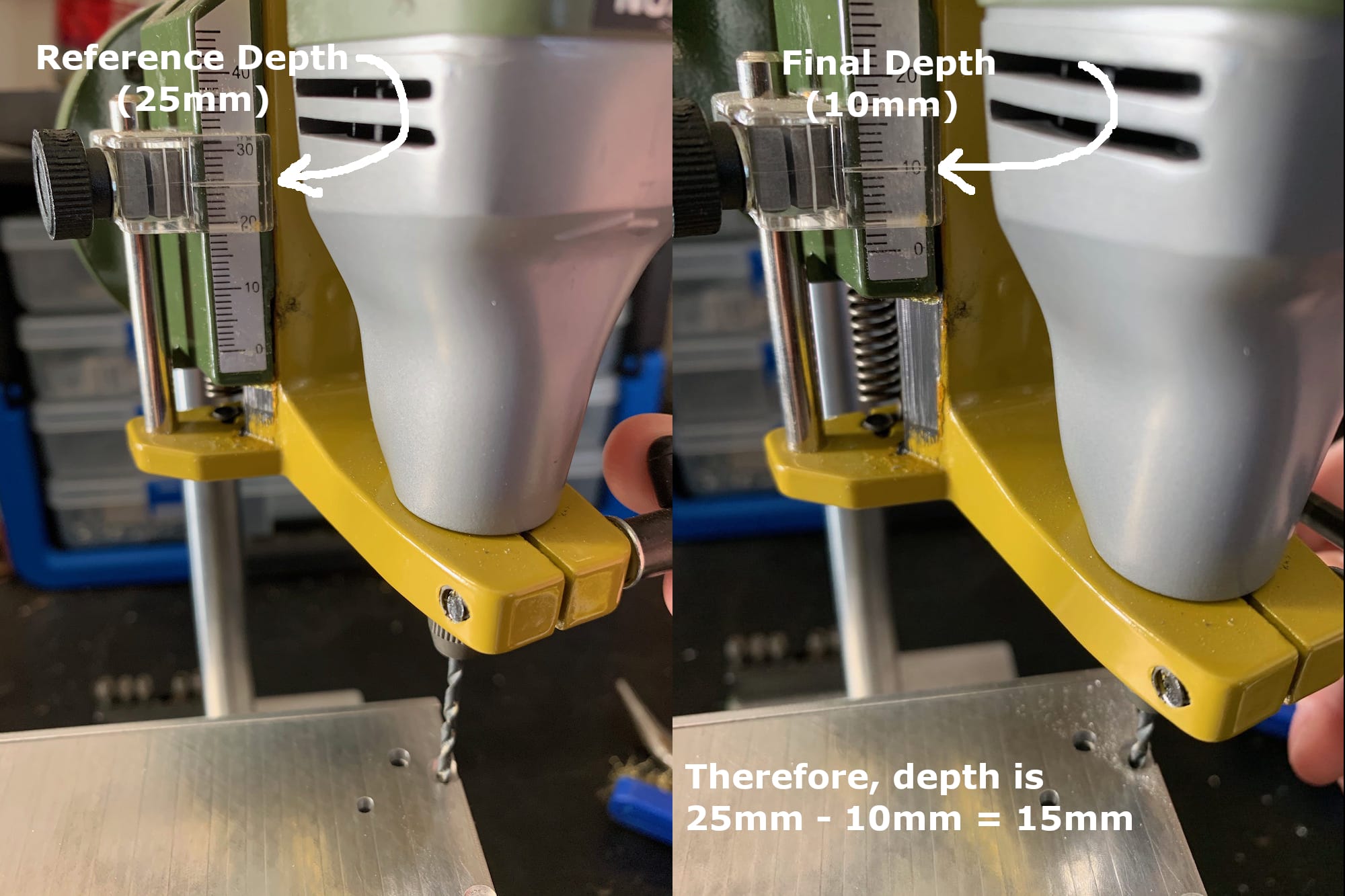
Fig 4.15-4. Hole depth measurement using the gauge
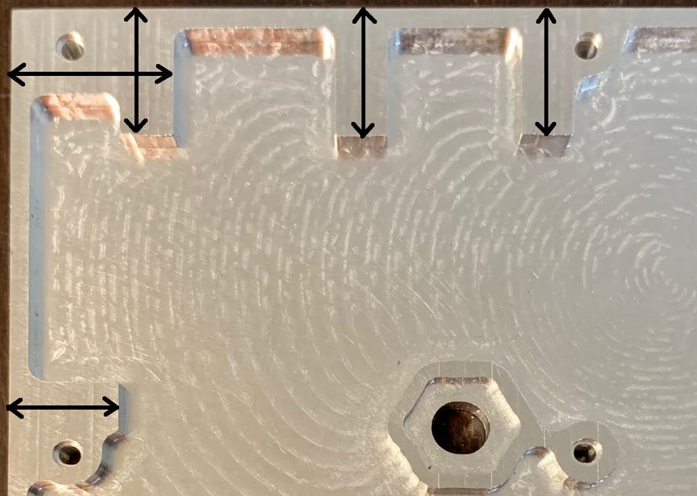
Fig 4.15-5. Thicker sections on the front face
Next, drill the six holes for the bottom face of the case. The three holes in the front face need to be ~ 15mm deep, and the three holes in the back face need to be ~ 12mm deep. After drilling the six bottom holes, carefully disassemble the case and remove the Nitto tape from the four edges of the front and back faces.
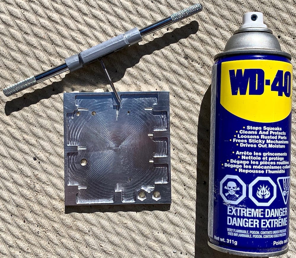
It is recommended for an inexperienced person to clamp the respective aluminum face piece within a bench vise before starting the tapping process. Install a 3mm (M3) x 0.5mm pitch tap into a tap handle/wrench. In a well-ventilated area, spray a small amount of WD-40 (or similar) liquid into one of the drilled holes in the front face. Slowly and carefully align the tap with the hole’s opening, ensuring that the tap is perpendicular (in both directions) to the surface containing the drilled hole. While applying moderate pressure on the tap in the direction of the hole, begin rotating the tap handle/wrench clockwise. The most challenging part of hand tapping these holes is getting the tap started within the drilled hole. Within a few turns from the start, it should become evident if the tap is beginning to make threads within the drilled hole.
Caution
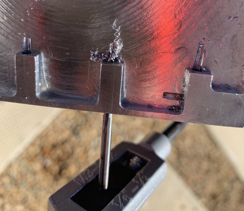
Manually tapping 3mm holes is time-consuming because the tap is very sensitive to breaking if too much rotational force is applied. It doesn’t take much force to break a 3mm tap. Once the tap feels ‘snug’ within the drilled hole, remove it and clean the swarf from its threads and from inside the drilled hole. Re-apply a small amount of WD-40 liquid in the drilled hole before beginning to deepen the tap from where you previously stopped. REMEMBER … SLOW AND STEADY!
After all the holes in the top and bottom edge surfaces of the front and back aluminum faces have been drilled and tapped, the case needs to be re-assembled using 3mm bolts to attach the top and bottom faces and Nitto tape to attach the left and right faces. Once re-assembled, the six holes in the left face and the six holes in the right face can be drilled using the Proxxon rotary tool. The holes for the left and right faces need to be ~ 12mm deep. At this depth, the outermost holes (of each set of three) will not be deep enough to go through the thicker sections of the aluminum. Tapping these holes will be slightly more difficult due to the drilled holes not forming open tunnels through the aluminum faces. After the holes in the left and right faces have been drilled, the case needs to be disassembled, and the holes tapped with the same M3 x 0.5mm pitch tap. Finally, the case needs to be re-assembled one more time to check the fit of the faces. Use 3mm bolts when attaching the faces. The four corners of the left and right faces will not perfectly align with the rounded edges on the top and bottom faces. Rather than creating a new CNC process for rounding over the corners of the left and right sides, which would be rather time-consuming, the corners can be quickly rounded over using a metal file. At most, there will be a couple of millimeters that need to be filed off.
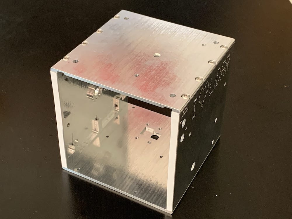
Fig 4.15-8. Top and bottom bolted, sides taped
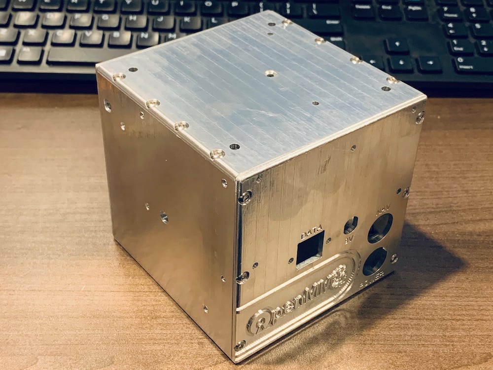
Fig 4.15-9. Case assembled with 3mm bolts
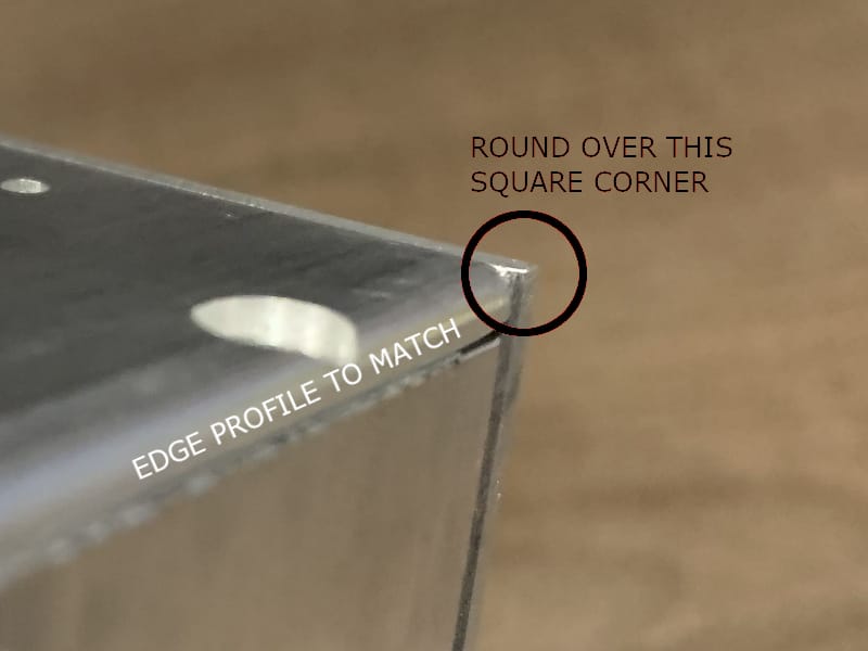
Fig 4.15-10. Corners need to be filed round
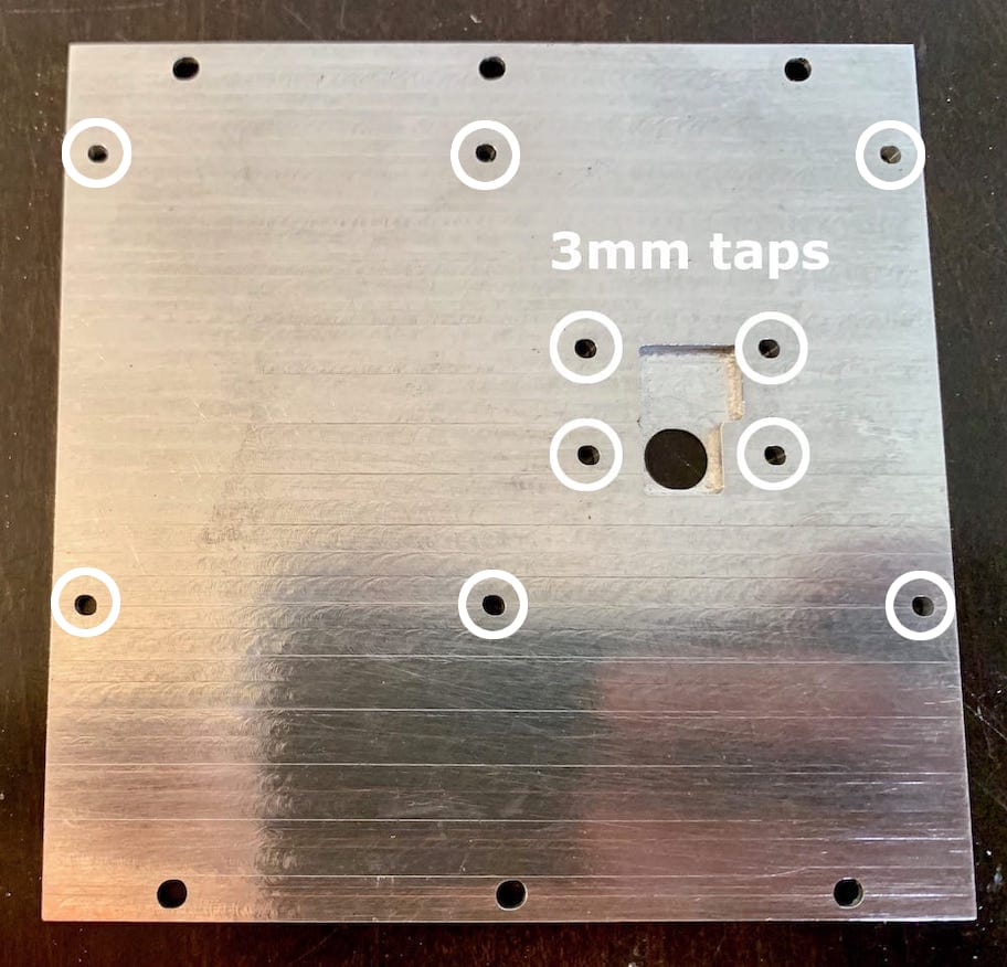
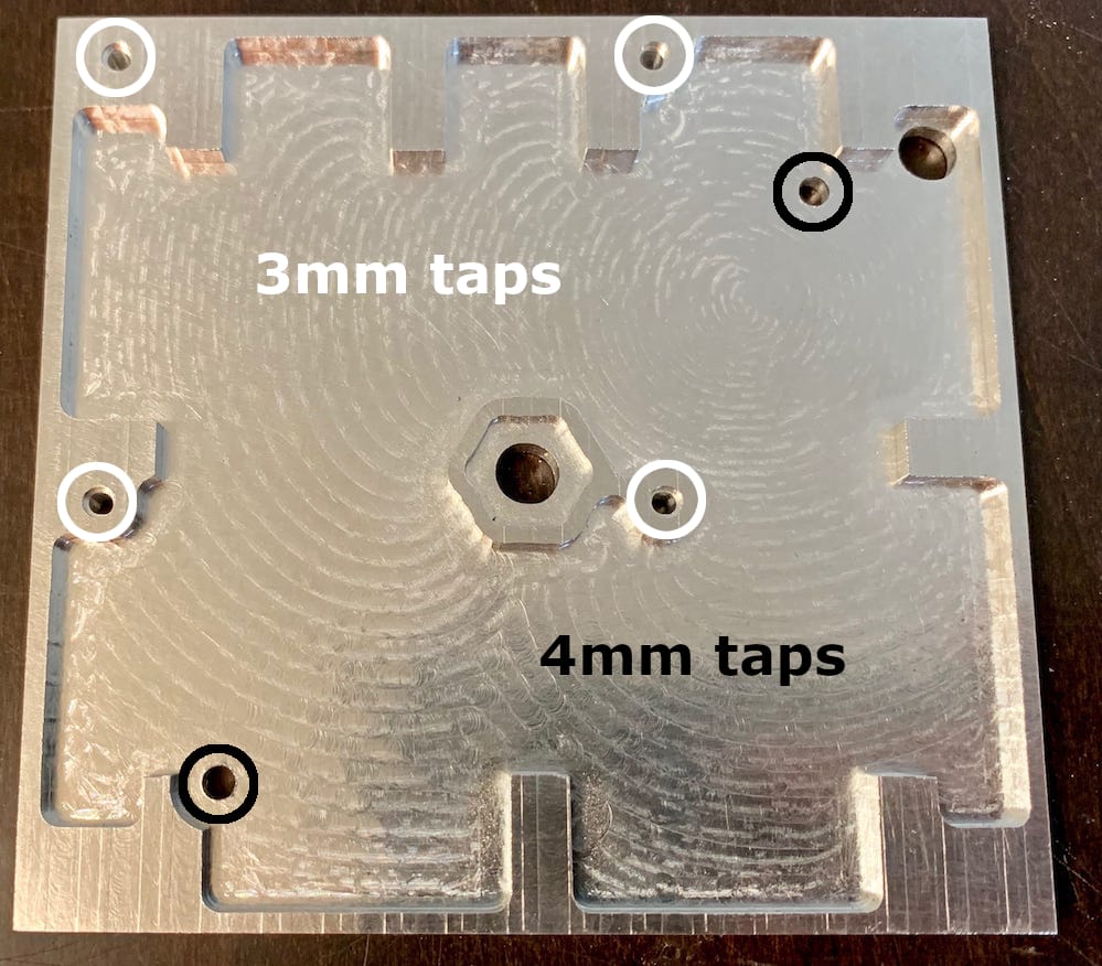
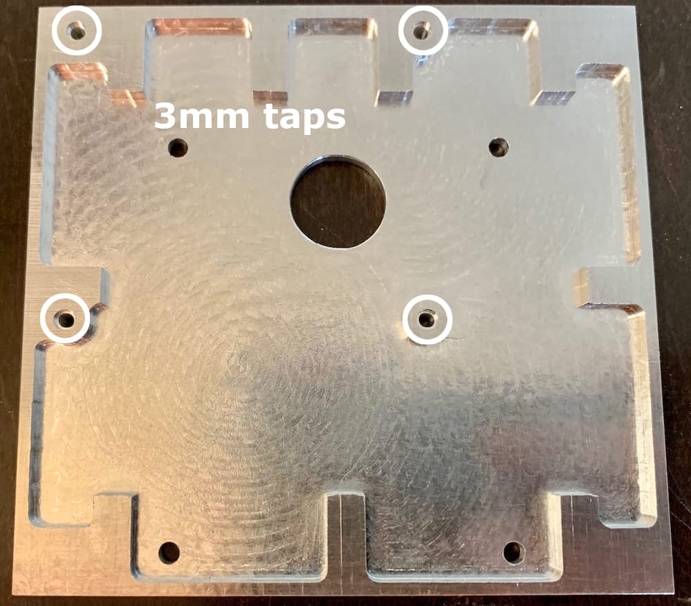
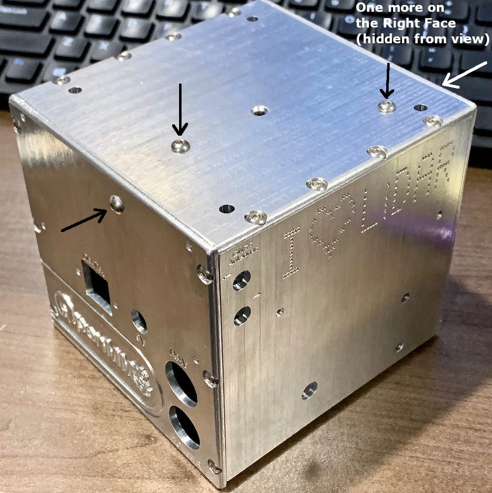
There are a few remaining holes on the front face and bottom face that require a 3mm tap. If you are using a Velodyne VLP-16 lidar sensor, and therefore manufacturing the VLP-16 specific front face, two additional holes require a 4mm tap. The figures below illustrate which holes need to be tapped.
4.15.2. GNSS Antenna Bracket Holes
The next task focuses on completing the manufacturing of the four GNSS antenna brackets. On the bottom of each bracket, write or scribe a unique ID number (i.e., 1,2,3,4). The recommended numbering has brackets 1 and 2 installed on the left face, towards the front and back faces, respectively. Likewise, brackets 3 and 4 are installed on the right face towards the front and back faces, respectively.
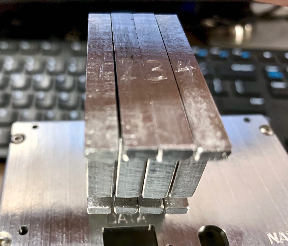
Fig 4.15-14. GNSS antenna bracket ID numbers
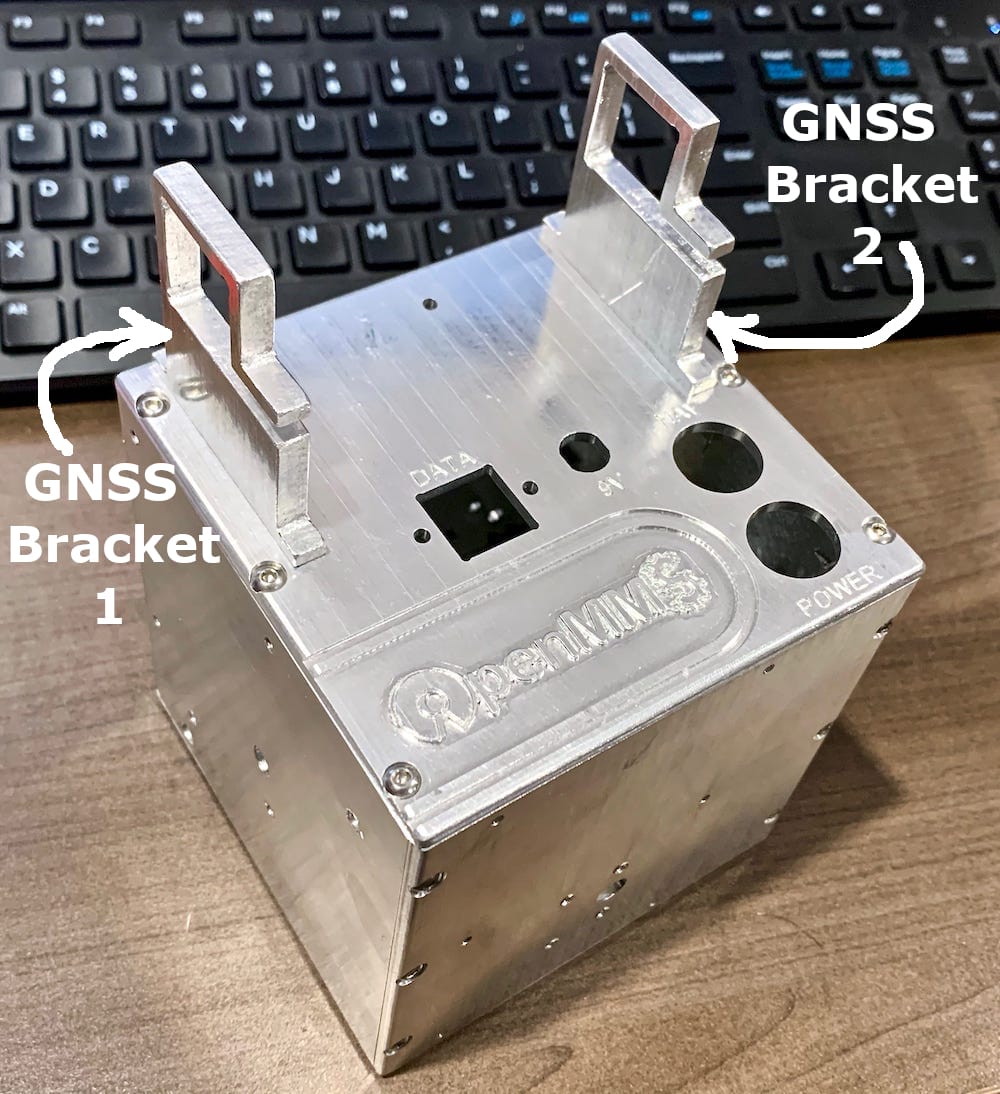
Fig 4.15-15. Left face GNSS antenna brackets
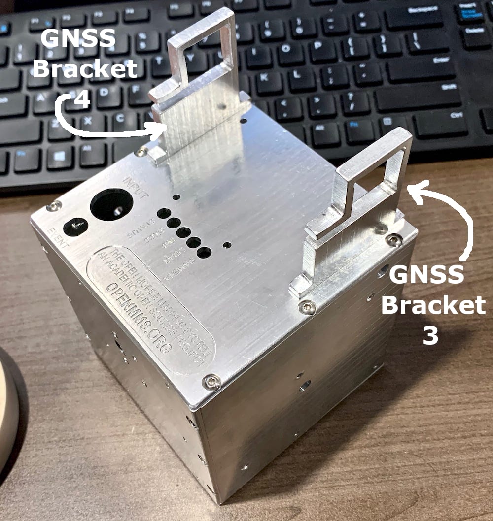
Fig 4.15-16. Right face GNSS antenna brackets
Next, remove the left and right faces from the assembled case. Place a piece of Nitto tape on the bottom surface of each GNSS antenna bracket, but be sure to leave the area underneath the mounting tabs free of tape. On the left face, align the top edge of the mounting tab on GNSS antenna bracket 1 with the ‘line’ where the top rounded edge of the left face starts, see Figure 4.15-18. Center the GNSS antenna bracket over the top holes near the front side of the left face. There should be a minimal gap between the front edge of the GNSS antenna bracket and the holes for assembling the case. Repeat this procedure for GNSS antenna bracket 2 on the rear side of the left face. Carefully flip the left face over and mark the hole locations on the backside of the mounting tabs on the GNSS antenna brackets. Remove the GNSS antenna brackets from the left face and remove the Nitto tape. Ideally, the marked hole locations should be on the center-line of the bracket. If the marked holes are not exactly in the center, that may still be ok. What is essential is that the marked holes form a line that is parallel to the edges of the bracket. If the line isn’t parallel, then the bracket will be installed with a twist in it, which will make it challenging to position the carbon fiber square tubing through both of the brackets. Repeat this process for all four GNSS antenna brackets.
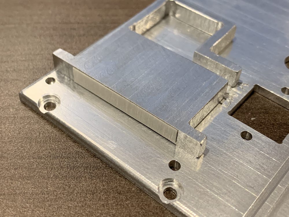
Fig 4.15-17. GNSS bracket with Nitto tape
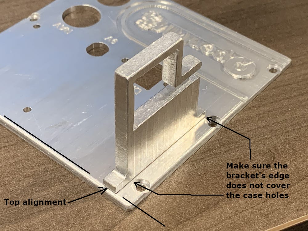
Fig 4.15-18. Bracket 1 in the correct position
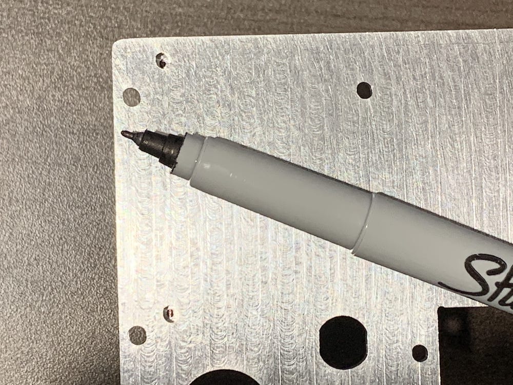
Fig 4.15-19. Marking holes inside the left face
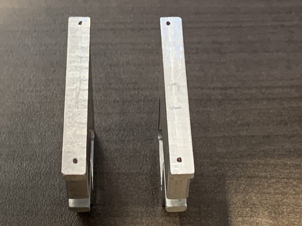
Fig 4.15-20. Marked holes to be drilled
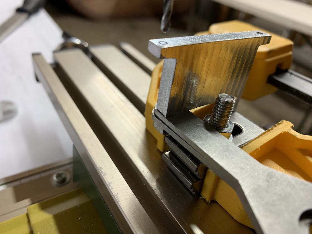
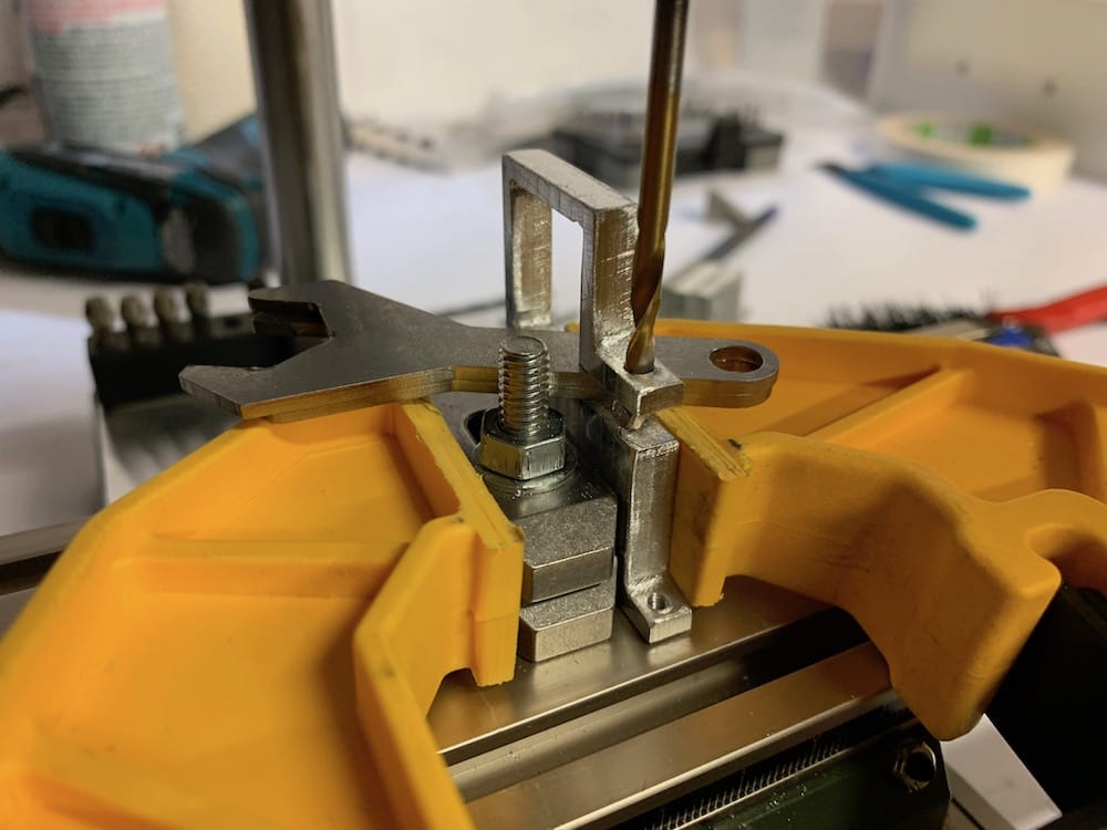
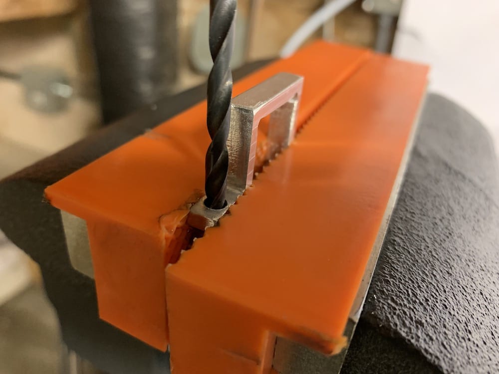
After the holes have been marked, as precisely as possible, drill the marked holes with the Proxxon Drill Press using a 3/32” drill bit. The GNSS antenna brackets will want to flex a little bit as you try to drill the holes. To help counteract this, wedge something within the opening of the brackets (e.g., a Bantam Tools Machine wrenches). Lastly, use the 3mm tap to create threads within the drilled holes.
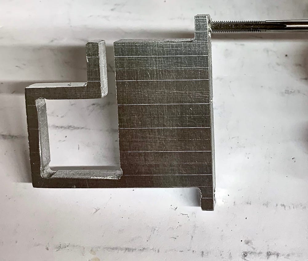
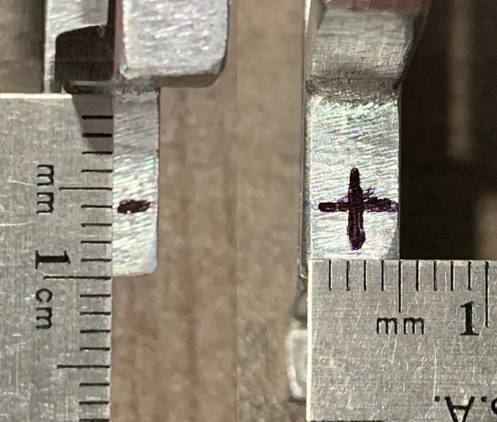
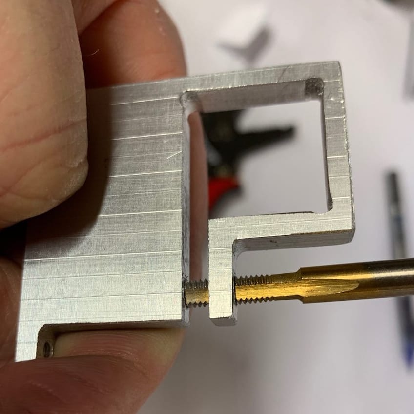
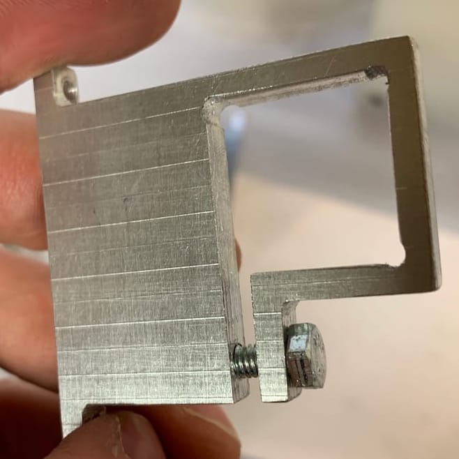
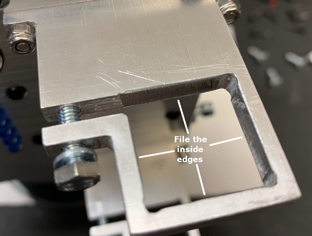
One final hole needs to be drilled and tapped into each of the GNSS brackets. On the closing tab, measure 4mm from the bottom edge, mark a line, and then find the midpoint across the closing tab and mark a line. The intersection of these lines is where the hole needs to be drilled, see Figure 4.15-23. Using the Proxxon Drill Press, install a 1/8” drill bit and drill a pilot hole to a depth of ~ 20mm (a 1/8” drill bit is the largest diameter bit that the Proxxon Rotary tool can use). Next, use a handheld electric drill to widen the 1/8” hole to a 9/64” hole (i.e., use a 9/64” drill bit in the handheld drill). Next, use a 3/16” drill to ONLY WIDEN THE TOP HOLE THROUGH THE CLOSING TAB. Next, use a 4mm tap to cut threads into the bottom part of the hole. Pass a 4mm hex bolt that is 10mm to 12mm in length through the wider top hole on the closing tab and thread it into the bottom hole. Lastly, ensure that the 20mm x 20mm carbon fiber square tubes fit through all four of the GNSS antenna brackets. The fit may be a bit tight, in which case the inside edges of square opening in the middle of the GNSS antenna brackets need to be filed down. It is not recommended to file down the carbon fiber tubes as they are relatively thin and can begin to crack and break if filed excessively.
4.15.3. Reinforcing Bracket Holes
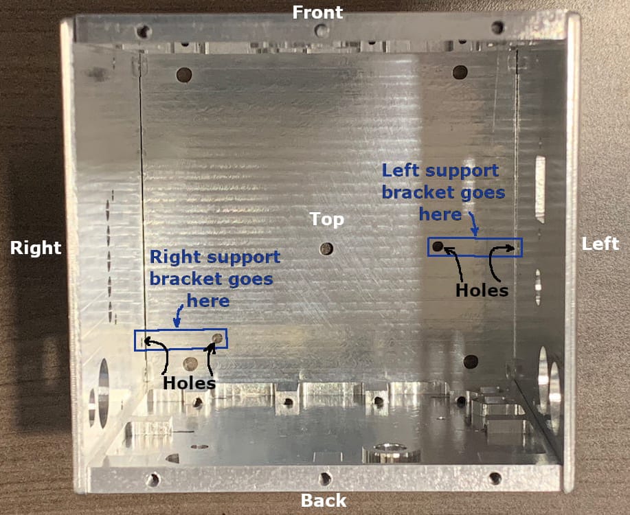
The next task focuses on completing the manufacturing of the two support brackets. Assemble the case using 3mm bolts, except leave the bottom face open. Mark/scribe the two support brackets with unique IDs. The recommended IDs are L and R. Using Nitto tape, if necessary, position the support brackets inside the case, as shown in the figure below. Carefully mark the position of the respective holes in the left and right faces ONLY on the support brackets. Remove the support brackets and drill the marked holes with the Proxxon Drill Press using a 3/32” drill bit. Cut threads into the drilled holes using a 3mm tap. Install the supports using 3mm bolts through the left and right faces. Once bolted into place, align the support brackets to cover their respective holes through the top face. Mark the hole locations, unbolt the brackets from the left and right faces, drill 3/32” holes, and cut threads using a 3mm tap. Reinstall the support brackets to ensure a correct fit.
4.15.4. Sony Bracket Holes
The next task focuses on completing the manufacturing of the Sony bracket. Remove the back face of the case, so it is free. First, with a handheld electric drill, carefully widen the left mounting tab on the Sony A6000 camera itself using a 3/32” drill bit (yes, you read this correctly!). Cut threads into this mounting tab using a 3mm tap. Next, insert a 1/2” long, 1/4” coarse threaded bolt and lock washer through the large hole on the back face. Thread the bolt into the mounting hole located on the bottom of the Sony A6000 camera, and gently tighten it until the camera feels secure on the back face but can still easily be rotated by hand (DO NOT OVERTIGHTEN THE 1/4” BOLT).
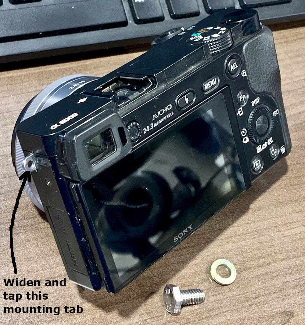
Fig 4.15-32. Adjust Sony mounting tab
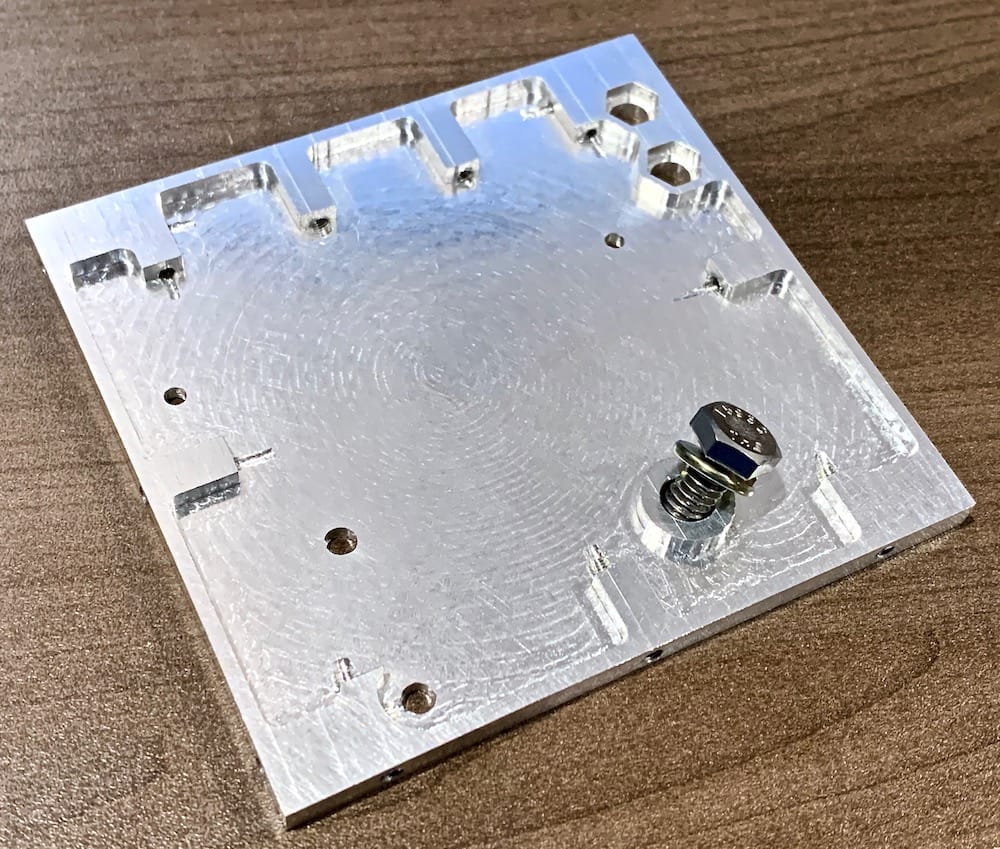
Fig 4.15-33. 1/4” coarse threaded bolt and lock washer
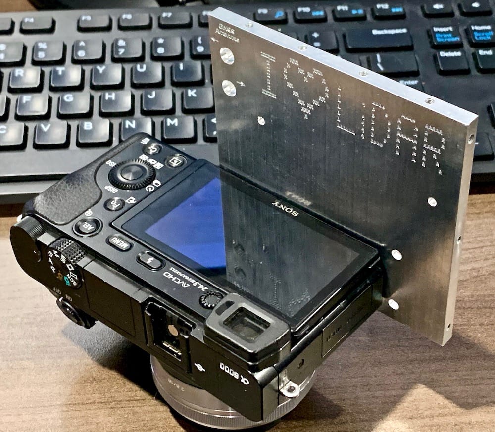
Fig 4.15-34. Sony A6000 attached to the back face
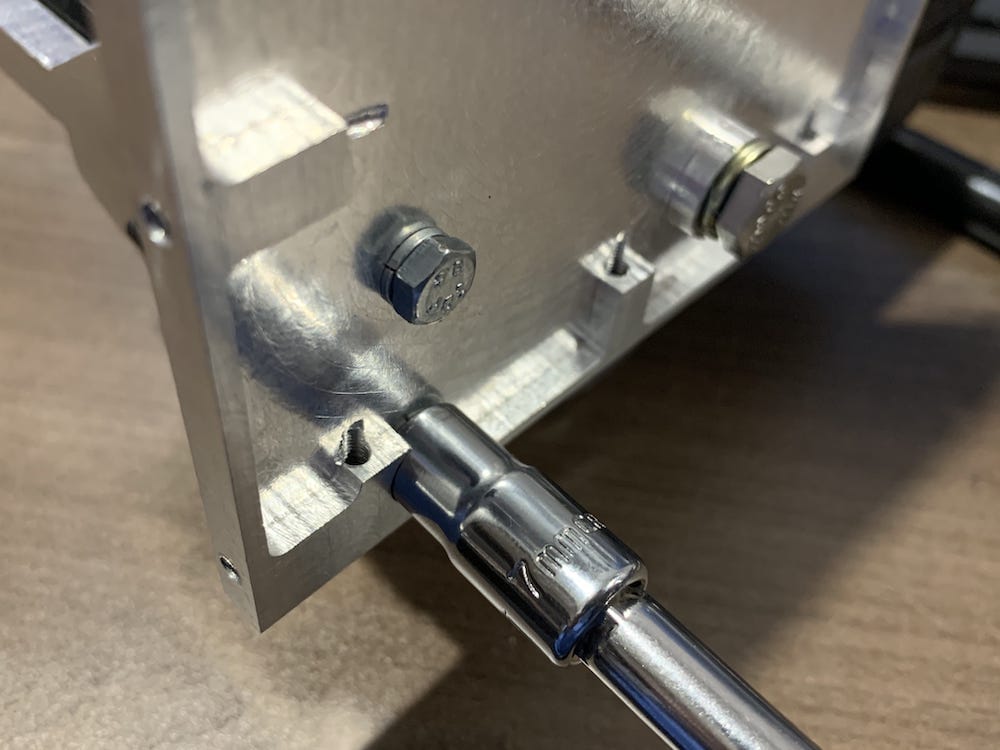
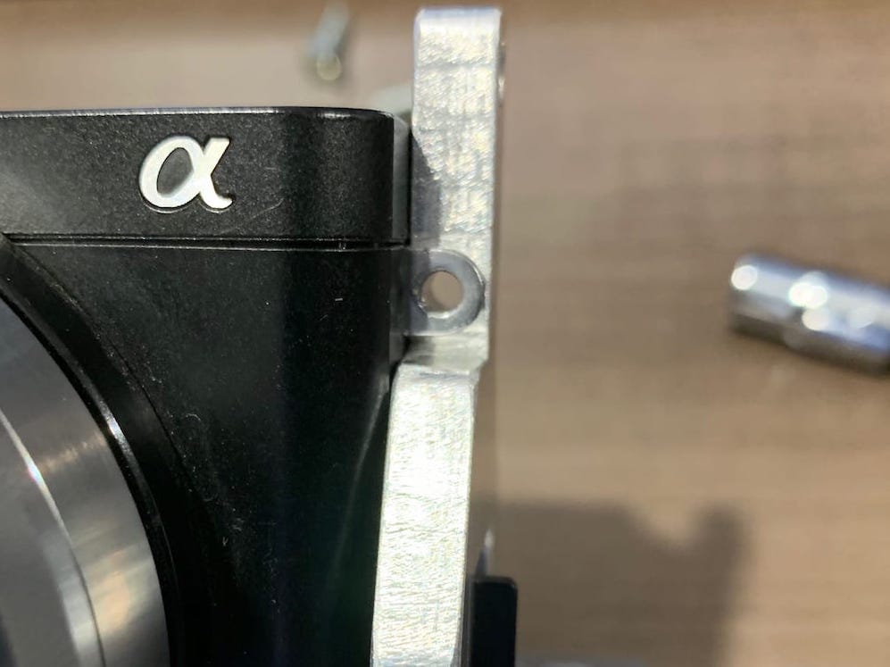
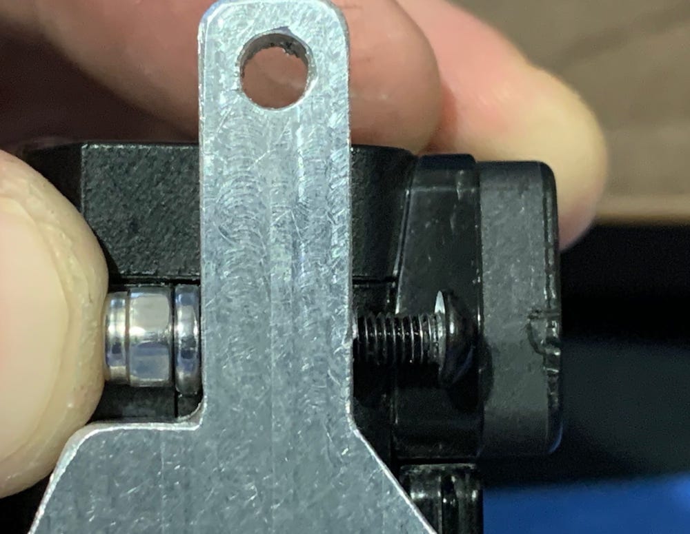
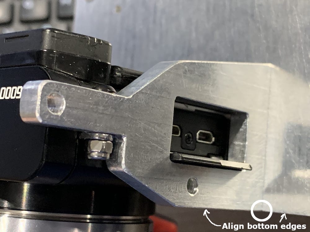
Next, position the Sony bracket tight against the left side of the camera. The bottom surface of the Sony bracket should be flush against the back face, in line with the two holes through the back face, and aligned with the bottom edge, see Figure 4.15-38. The left mounting tab of the Sony A6000 camera should be touching the ‘underside’ of the Sony bracket. Also, ensure that the HDMI/Multi connection panel on the camera is open and fits through the opening in the bracket. Next, mark the two holes’ positions through the back face, on the bottom surface on the bracket. Using the Proxxon Drill Press with a 1/8” drill bit, drill the two marked holes to a depth of ~ 12mm. Using a handheld electric drill with a 9/64” drill bit, widen the 1/8” pilot holes. Cut threads into the holes using a 4mm tap. Attach the Sony bracket to the back face using 4mm by 10mm length bolts and lock washers. Next, CAREFULLY tighten the 1/4” bolt until it is firmly snug. The camera’s mounting tab touching the underside of the Sony bracket will help resist the camera from rotating while the 1/4” bolt is tightened (though the camera may turn a little bit, and this is ok). Next, mark the position of the mounting tab hole on the underside of the Sony bracket. Remove the Sony bracket from the back face. Using the Proxxon Drill Press with a 1/8” drill bit, drill the marked hole through the Sony bracket. THIS HOLE IS NOT TAPPED! Reattach the Sony bracket to the back face using the 4mm bolts and lock washers. Insert a 3mm bolt ~ 14mm in length through the drilled hole on the Sony bracket’s topside. Position a Nyloc nut directly under the mounting tab and thread the bolt through the Sony A6000 camera mounting tab and then through the Nyloc nut.
4.16. Part Cleaning and Finishing
The final task in this step focuses on cleaning and finishing all the aluminum parts to ensure that no loose pieces of metal swarf remain that may damage the electronic components inside the case. Sticking with the desktop manufacturing only approach, no ultrasonic cleaners, tumble deburring machines, etc. were used in this task. However, if you have access to these cleaning and finishing solutions (and know what you are doing), they certainly can be used.
First, it is recommended to affix ALL of the hardware components (i.e., bolts, standoffs, pushbuttons, Lemo connectors, etc.) to the six faces of the case. The intention is to make sure the hardware fits within the machined or manually drilled and tapped holes of the case. Some of the machined holes (i.e., holes created by the Bantam Tools Machine) may be a bit snug, and hence the respective bolts do not easily fit into the holes, but rather require the bolts to be threaded in using a driver. Ideally, all the machined holes should allow for bolts to slide easily, though not loosely, through the holes and not requiring them to be threaded in using a driver. The figures below illustrate which hardware components go where for each face. BLUE CIRCLED BOLTS NEED TO BE ABLE TO SPIN FREELY WITHIN THEIR RESPECTIVE HOLES. The red circled bolts are going through threaded holes, and therefore SHOULD NOT SPIN FREELY. It does not matter if the orange circled bolts spin freely or not.
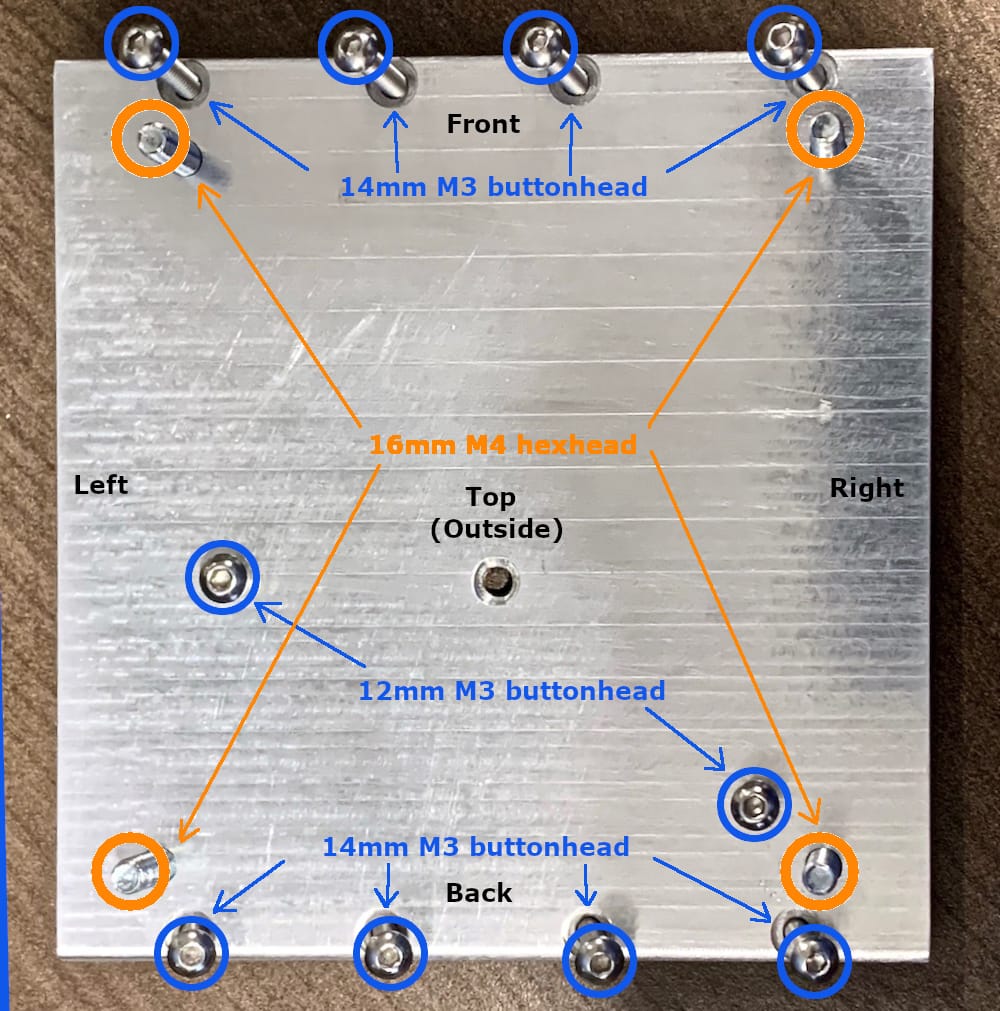
Fig 4.16-1. Top face hardware
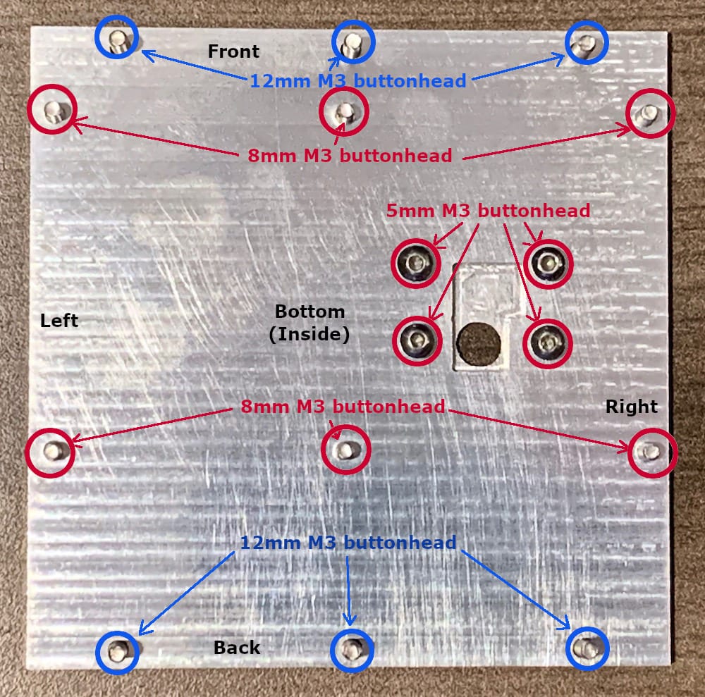
Fig 4.16-2. Bottom face hardware
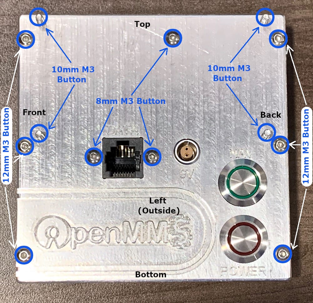
Fig 4.16-3. Left face hardware
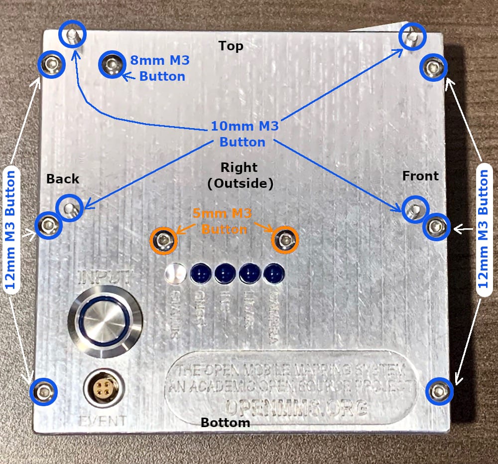
Fig 4.16-4. Right face hardware
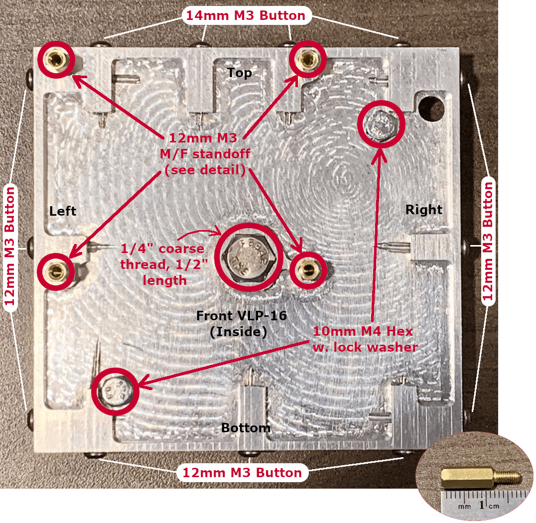
Fig 4.16-5. Front face (VLP-16) hardware
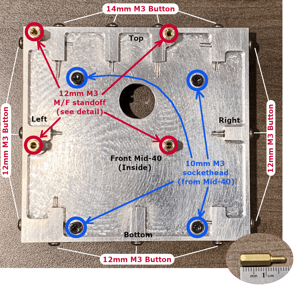
Fig 4.16-6. Front face (MID-40) hardware
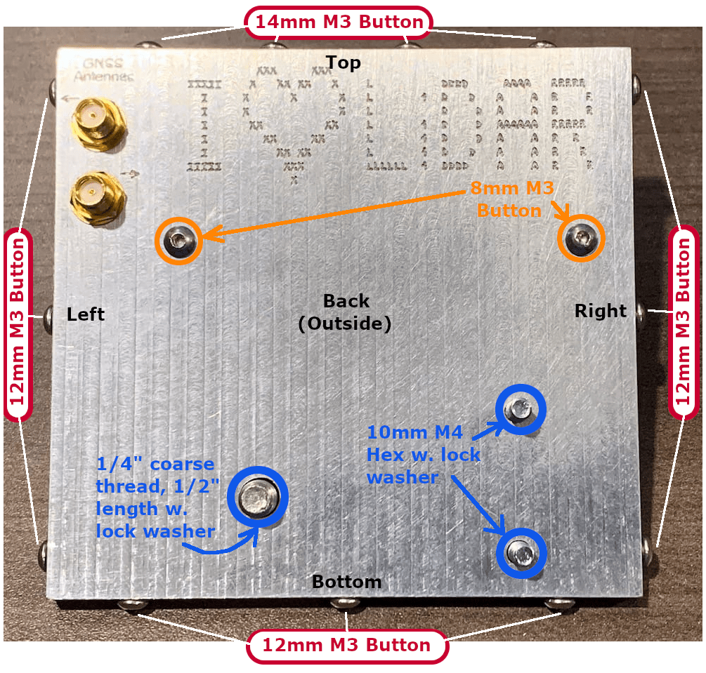
Fig 4.16-7. Back face hardware
Ensure that all the hardware fits within the respective holes, then take it all apart until the six faces are separated and free of the hardware. The next task is to repeat the instructions discussed in the After Machining step. Pay close attention to the starting point and ending point (if visible) of all the manually drilled holes. Look for small pieces of aluminum that appear loosely attached to the part and remove them. Using compressed air to blow through the drilled and tapped holes can help remove unwanted (and potentially damaging) minute pieces of aluminum hidden within the holes. Take your time with this step; attention to detail is important. After completing this step, no more machining or adjusting of the aluminum parts will be performed! The final task is to thoroughly clean all the parts using warm water and a mild cleaning/degreasing solution. Scrub all the surfaces of the parts, rinse with clean water, and leave to air dry.
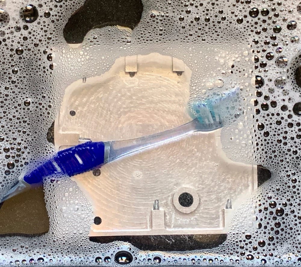
Fig 4.16-8. Thoroughly scrub each aluminum part
CONGRATULATIONS!
YOU HAVE NOW FINISHED MANUFACTURING THE ALUMINUM PARTS!
5. Printed Circuit Boards Manufacturing
5.1. Overview
There are a total of three printed circuit boards that need to be manufactured using the Bantam Tools Machine. The LED, APX-18, and R.Pi boards are machined out of double-sided PCB blanks. Each PCB requires the use of the same three End Mills (1/16” Flat, 1/32” Flat, 0.005” PCB Engraving). Pay close attention to the required End Mill for each milling operation and ensure that the Bit Fan is always installed on each End Mill. The Bantam Tools Machine should be cleaned of dust and removed PCB materials whenever safely possible. The Fine Dust Collection System or Vacuum Port performance upgrades are highly recommended.
The reader is strongly encouraged to work through the Bantam Tools Light Up PCB Badge - Getting Started Project before proceeding with manufacturing the OpenMMS PCBs. The Getting Started Project provides excellent explanations, does and don’ts, and other valuable information on PCB milling using the Bantam Tools Machine.
Autodesk Eagle software was used to design the PCBs. All of the design information and digital files are included below for each PCB. Each PCB has two sets of design information. The 1st set is for a design that can be manufactured by the end-user using the Bantam Tools Machine. The PCB tables below include the design information and manufacturing steps for creating the PCBs using the Bantam Tools Machine. The 2nd set of designs for each PCB contains the information that can be sent to a commercial PCB manufacturer. These designs are included in the Commercially Made PCBs section below. The design differences are the trace widths, via sizes, use of plated through holes, and some hole sizes. The Bantam Tools PCBs do not use plated through holes. The PCBs’ vias need to be manually soldered, and the boards do not have a conformal coating. Therefore, precise soldering is an essential skill required to produce the PCBs successfully.
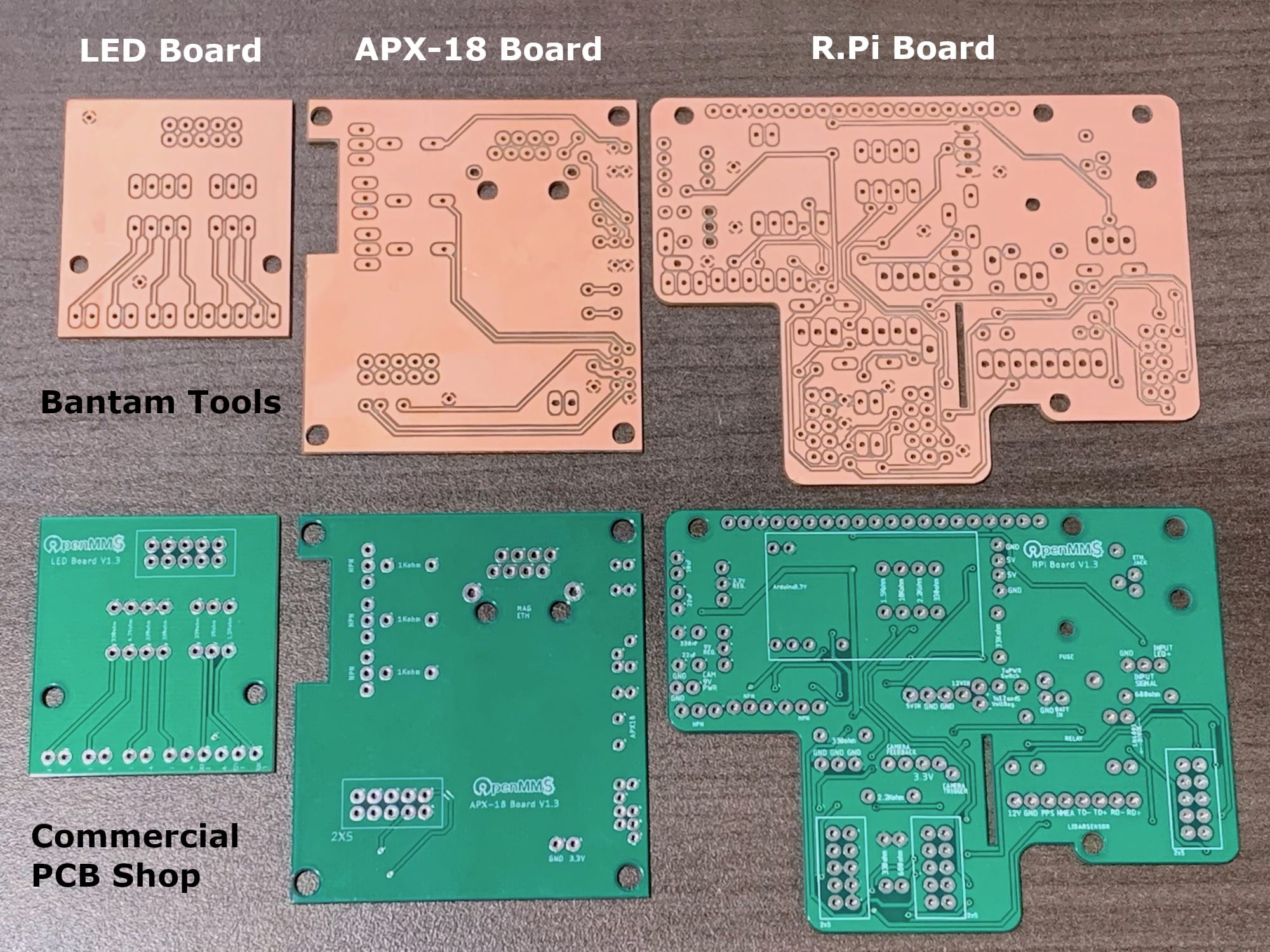
Fig 5.1-1. OpenMMS Printed Circuit Boards
5.2. Instructions
Manufacturing PCBs using the Bantam Tools Machine is more straightforward than the aluminum parts. However, the final manufacturing quality of the PCBs is much more critical than for the aluminum parts. All milling operations are performed using the 3rd Bantam Tools Machine Setup (BTMS). See the previous Bantam Tools Machine Setups section for details. Strong double-sided tape is required to hold the PCB blanks while being machined. Special care needs to be used when removing the PCBs from the spoilboard. Using isopropyl alcohol to release the strong tape is a MUST, or you run the risk of damaging the PCB while trying to remove it from the machine!
All three PCBs can be squeezed onto one double-sided PCB blank, and therefore manufactured at the same time. It is crucial to pay close attention to the Bantam Tools Software Configuration settings for each PCB milling operation as there are NO individual GCODE files used for milling the PCBs. Instead of GCODE files, the Eagle produced board design files (.brd files) are used directly within the Bantam Tools software, and the software generates all the milling commands based on the design. There are two top PCB operations and three bottom PCB operations required to complete each board.
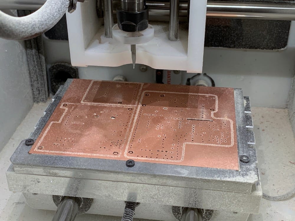
Fig 5.2-1. All three PCBs being milled (forgot to turn on the vacuum, oops)
Because all three PCBs can be milled from the same double-sided PCB blank, the same type of milling operation (i.e., holes, or traces, or outlines) can be performed sequentially for each PCB. Continuous milling operations can be accomplished by selecting the same type of milling operation for all three PCBs within the Bantam Tools software and then clicking the ‘Mill All Visible’ button at the bottom of the right side column. Equivalently, you can perform ALL the 1st milling operations on the three PCBs, then ALL the 2nd milling operations, until lastly ALL the 5th milling operations are completed. The figure below illustrates the Bantam Tools software Part Placement settings for each PCB that allows all of them to fit on a single PCB blank.
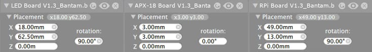
Fig 5.2-2. Bantam Tools software part placement settings for the PCBs
Attention
For those interested in viewing/editing the Autodesk Eagle projects for the PCBs, you will need to download the OpenMMS Eagle Libraries and Design Rules and add them to your local Eagle environment. The author of this documentation is a beginner user of Autodesk Eagle software, and therefore the PCB designs and schematics are simplistic and likely appear unconventional. Community contributions in this area of the project would be most welcomed!
5.3. Commercially Made PCBs (optional)
If a reader is interested in having the OpenMMS PCBs manufactured by a commercial printed circuit board shop, the following design information for each PCB should be used. Included within these design information zip files are:
Autodesk Eagle project file.
Eagle schematic file (.sch)
Eagle board file (.brd)
CAMOutputs directory, this contains all the Gerber files that a commercial PCB manufacturer will require.
PDF file showing the electrical schematic for the PCB
PDF file showing the layout of the PCB (both sides)
Table H11: Production Version PCBs Design Files
PRODUCTION VERSION
PCB DESIGN FILES2D/3D Viewer
5.4. LED Board
Table H12: LED Board Design and Manufacturing Files
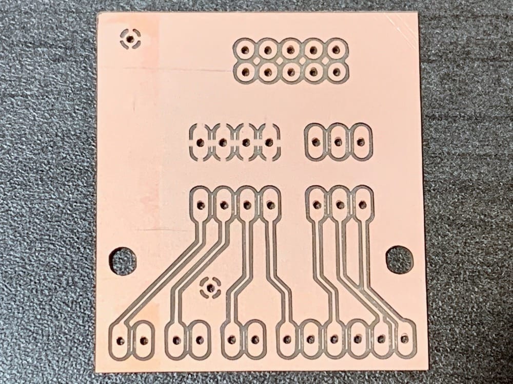
Fig 5.4-1. LED Board (Top)
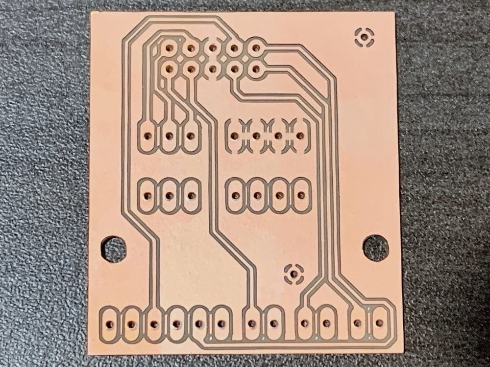
Fig 5.4-2. LED Board (Bottom)
Version: 1.3
Quantity: 1
Material:
FR-1 Double-sided PCB Blank
End Mills Required:
Blank Dimensions:
127.0mm x 101.6mm x 1.6mm
1/16” Flat End Mill (16F)
1/32” Flat End Mill (32F)
0.005” PCB Engraving Bit (5E)
BANTAM VERSION PCB DESIGN:
2D/3D Viewer:
MILLING OPERATIONS
Order
Purpose
BTMS
Install @
End Mill
Eagle Board File:
Bantam Tools Software Configurations
1
2
3
4
5
Traces
Holes
Holes
Traces
Outline
3
3
3
3
3
Top
Top
Bottom
Bottom
Bottom
5E
32F
32F
5E
16F
LED Board V1.3_Bantam.brd
SAME
SAME
SAME
SAME
5.5. APX-18 Board
Table H13: APX-18 Board Design and Manufacturing Files
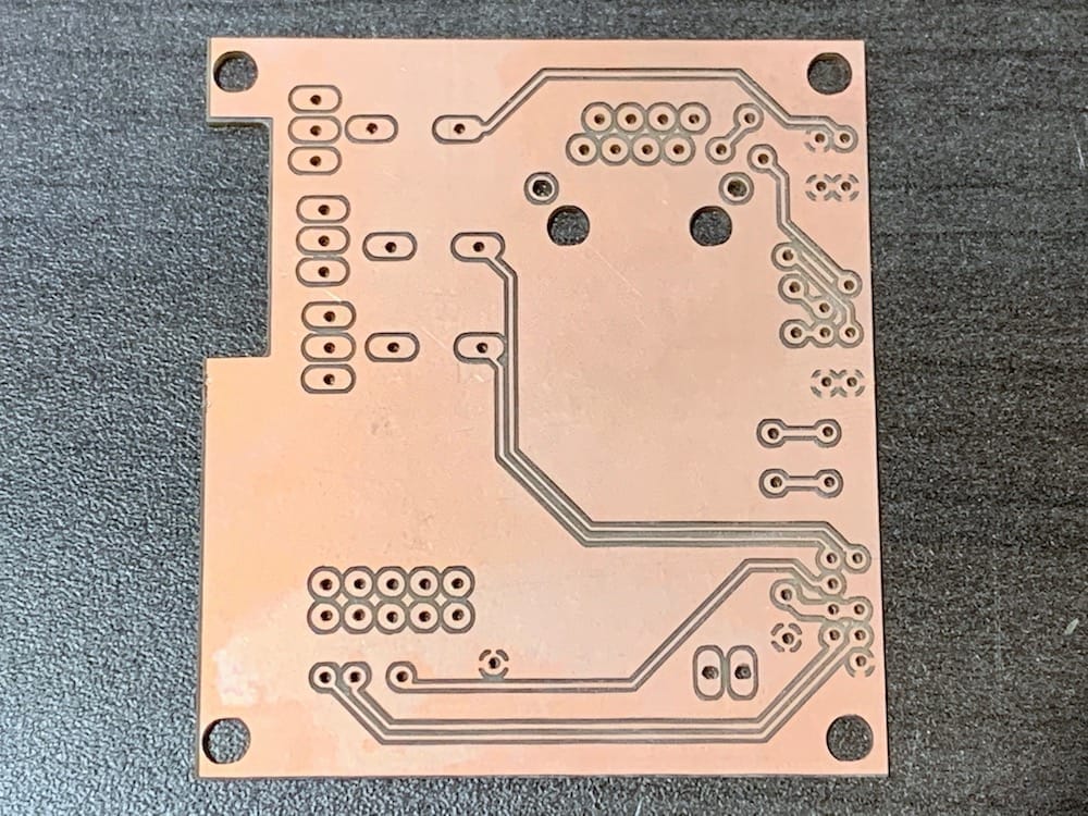
Fig 5.5-1. APX-18 Board (Top)
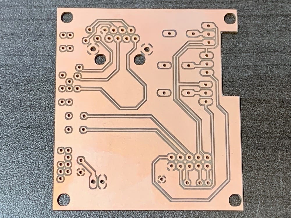
Fig 5.5-2. APX-18 Board (Bottom)
Version: 1.3
Quantity: 1
Material:
FR-1 Double-sided PCB Blank
End Mills Required:
Blank Dimensions:
127.0mm x 101.6mm x 1.6mm
1/16” Flat End Mill (16F)
1/32” Flat End Mill (32F)
0.005” PCB Engraving Bit (5E)
BANTAM VERSION PCB DESIGN:
2D/3D Viewer:
MILLING OPERATIONS
Order
Purpose
BTMS
Install @
End Mill
Eagle Board File:
Bantam Tools Software Configurations
1
2
3
4
5
Traces
Holes
Holes
Traces
Outline
3
3
3
3
3
Top
Top
Bottom
Bottom
Bottom
5E
32F
32F
5E
16F
APX-18 Board V1.3_Bantam.brd
SAME
SAME
SAME
SAME
5.6. RPi Board
Table H14: RPi Board Design and Manufacturing Files
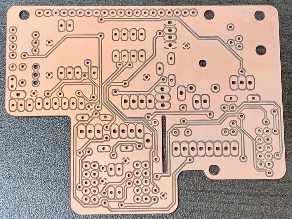
Fig 5.6-1. RPi Board (Top)
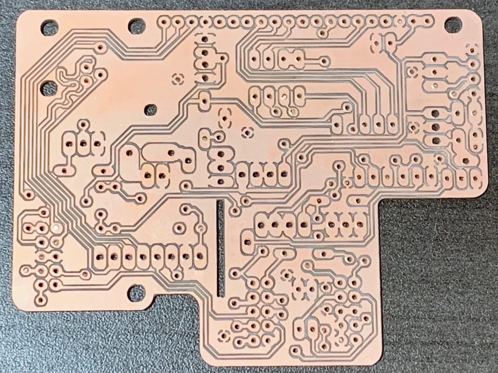
Fig 5.6-2. RPi Board (Bottom)
Version: 1.3
Quantity: 1
Material:
FR-1 Double-sided PCB Blank
End Mills Required:
Blank Dimensions:
127.0mm x 101.6mm x 1.6mm
1/16” Flat End Mill (16F)
1/32” Flat End Mill (32F)
0.005” PCB Engraving Bit (5E)
BANTAM VERSION PCB DESIGN:
2D/3D Viewer:
MILLING OPERATIONS
Order
Purpose
BTMS
Install @
End Mill
Eagle Board File:
Bantam Tools Software Configurations
1
2
3
4
5
Traces
Holes
Holes
Traces
Outline
3
3
3
3
3
Top
Top
Bottom
Bottom
Bottom
5E
32F
32F
5E
16F
RPi Board V1.3_Bantam.brd
SAME
SAME
SAME
SAME
5.7. Support Board
An additional ‘part’ is also machined out of PCB material. It does not contain any electronic circuitry, but once installed in the case its copper-covered side(s) will act as a ground plane. This ‘part’ is called the Support Board and it can be machined out of a single-sided PCB blank (or a double-sided PCB blank if that is all you have). There is a single GCODE file for creating the Support Board using a 1/8” Flat End Mill.
Table H15: Support Board Design and Manufacturing Files
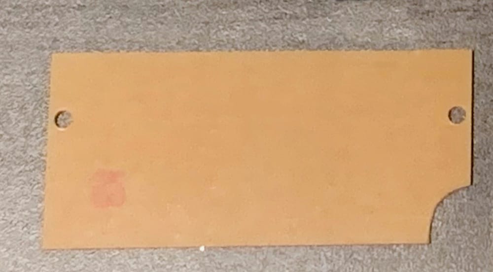
Fig 5.7-1. Support Board (Single-sided PCB)
Version: 1.3
Quantity: 1
Material:
FR-1 Single (or Double) sided PCB Blank
End Mills Required:
Blank Dimensions:
127.0mm x 101.6mm x 1.6mm
1/8” Flat End Mill (8F)
Fusion 360 File(s):
MILLING OPERATIONS
Order
Purpose
BTMS
Install @
End Mill
GCODE Files:
Bantam Tools Software Configurations
1
Cut
3
Top
8F
5.8. After Milling
It is recommended to use a metal file to gently round the sharp 90 degree edges of the Support Board after being milled by the Bantam Tools Machine. Once installed, several power wires run across the edges of the Support Board. The rounded edges prevent the wires from having their protective sheathing cut, potentially causing a short circuit. Next, carefully examine both sides of the printed circuit boards and identify small pieces of copper that could come free. Using the pinpoint tip of an X-Acto knife, carefully remove these pieces of copper. Lastly, it is recommended to scour both sides of the printed circuit boards lightly. A coarse plastic brush works well for this task. The goal is to remove any loose pieces of copper from the printed circuit boards. These pieces of copper could cause electrical damage (i.e., create short-circuits) on the sensitive (and costly) sensors and components inside the case.
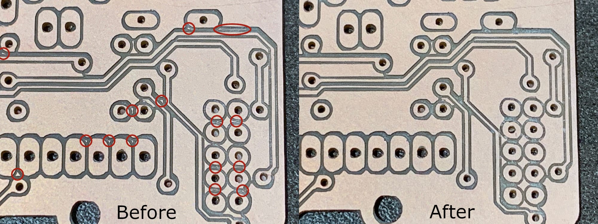
Fig 5.8-1. PCB area before and after removing loose/potentially loose pieces of copper
CONGRATULATIONS!
YOU HAVE NOW FINISHED MANUFACTURING THE PRINTED CIRCUIT BOARDS!
6. Carbon Fiber Parts Manufacturing
Danger
Machining parts from carbon fiber material can create potentially hazardous carbon fiber dust in the air. It is the responsibility of the person(s) using these instructions to produce their own (i.e., the manufacturer of an) OpenMMS sensor, to ensure that satisfactory air quality requirements are met or exceeded, during any process discussed within these instructions when working with carbon fiber material.
6.1. Overview
There are 2 carbon fiber parts that need to be manufactured using the Bantam Tools Machine. The parts are identical and are used as ground planes for the GNSS Antennas connected to the Applanix APX-18 GNSS-INS sensor. The parts are machined out of 2mm thick carbon fiber plate, using a 1/16” Flat End Mill. Ensure that the Bit Fan is installed on the End Mill. The Fine Dust Collection System performance upgrade is HIGHLY RECOMMENDED. As a minimum, the Vacuum Port performance upgrade should be used to remove as much potentially hazardous carbon fiber dust as possible.
6.2. Instructions
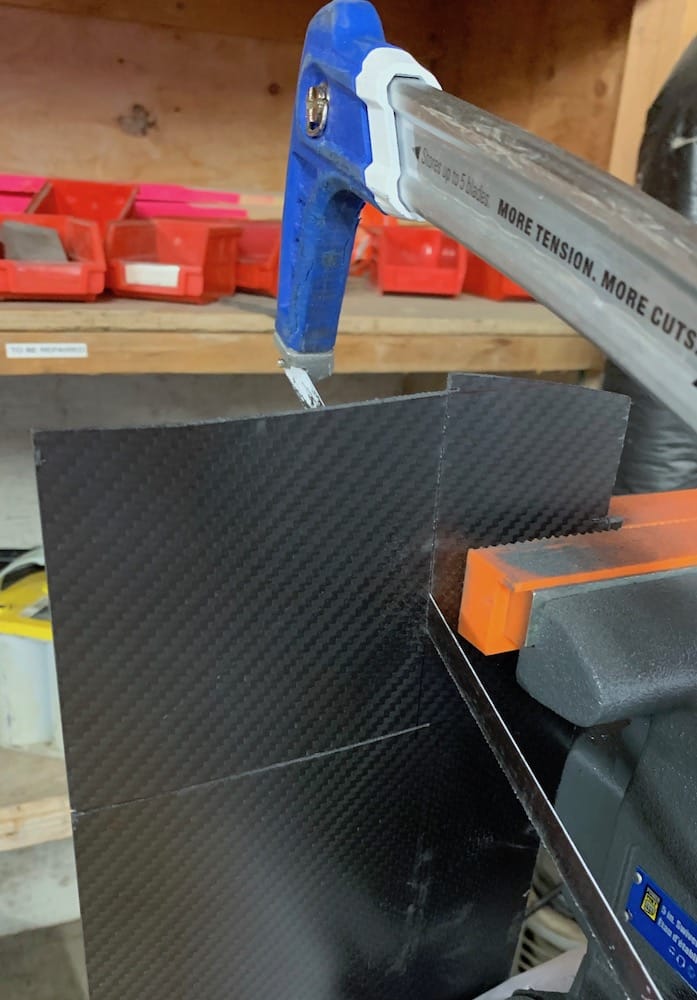
Firstly, the 2mm thick carbon fiber plates need to be manually cut into 105mm x 105mm (min.) to 110mm x 110mm (max.) square pieces. Using a bench vise and a sharp hacksaw can make this an easy task. Mount the carbon fiber blank into the Bantam Tools machine using the 4th Bantam Tools Machine Setup (BTMS) and install a 1/16” Flat End Mill into the machine. Run the single milling operations to manufacture the GNSS Antenna ground plane. Repeat this procedure to create a total of two ground planes.
6.3. Ground Plane
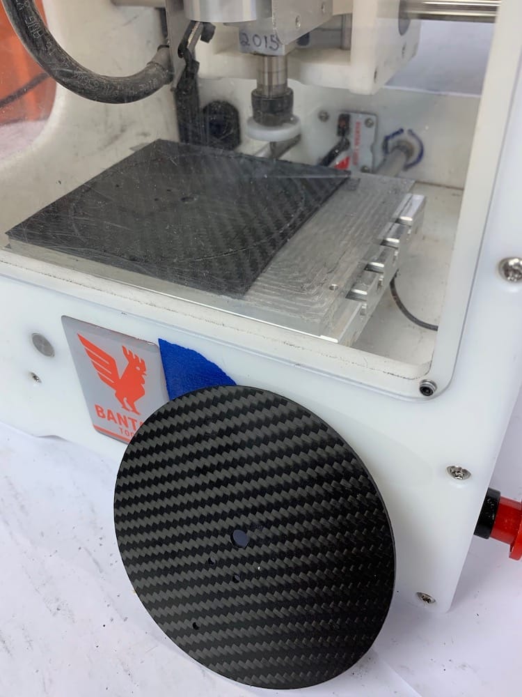
Table H16: Ground Plane Design and Manufacturing Files
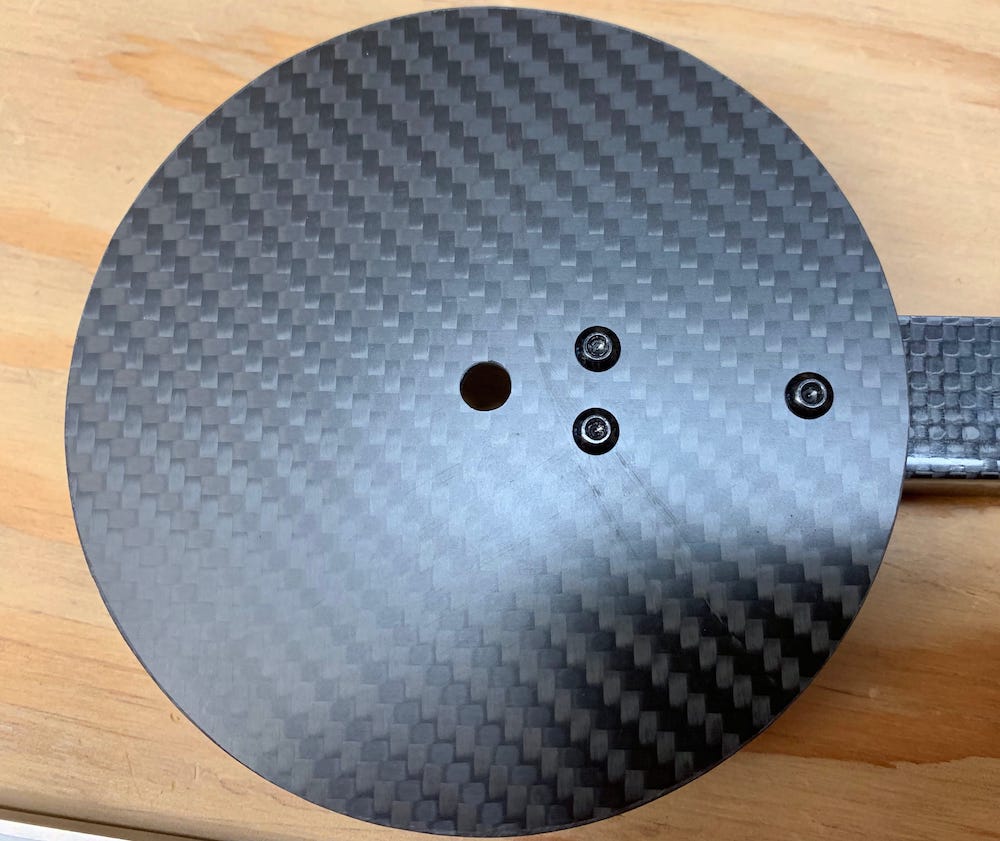
Fig 6.3-1. Carbon Fiber Ground Plane
Version: 1.3
Quantity: 2
Material:
2mm thick carbon fiber plate
End Mills Required:
Blank Dimensions:
105mm x 105mm (min.) to 110mm x 110mm (max.) x 2mm
1/16” Flat End Mill (16F)
Fusion 360 File(s):
MILLING OPERATIONS
Order
Purpose
BTMS
Install @
End Mill
GCODE Files:
Bantam Tools Software Configurations
1
Cut
4
Arbitrary
16F
6.4. After Milling
It is recommended to use a metal file to gently round the sharp 90 degree edges of the Ground Planes after being milled by the Bantam Tools Machine. Carbon fiber can be very sharp once cut. It is also electrically conductive, so it is crucial to make sure that the GNSS antenna cables do not rub against any sharp carbon fiber edges.
CONGRATULATIONS!
YOU HAVE NOW FINISHED MANUFACTURING THE CARBON FIBER PARTS!
7. Cables Assembly
7.1. Overview
There is a total of eleven cables of five different types that need to be assembled. Seven of the cables are installed inside the case, while the other four cables are used outside the case to connect specific components. Custom length ethernet cables with modified RJ45 connector ends need to be made due to the extremely tight fit of these cables inside the case. Therefore, RJ45 connector ends, Cat5/6 ethernet cable, and an RJ45 crimping tool are required.
7.2. 10-wire Ribbon Cables
A total of three 10-wire ribbon cables need to be assembled. Two of the cables are identical and can be installed between the respective PCBs without any attention to which end goes where. The remaining cable only has a connector on one end, while the other end is directly soldered to the respective components on the Left Face of the case (see the Left Face Assembly section for the details).
The following components are needed to assemble the three 10-wire ribbon cables.
5 @ 10-wire male housing/female pin connectors
3 @ 10-wire ribbon cable, 9cm in length
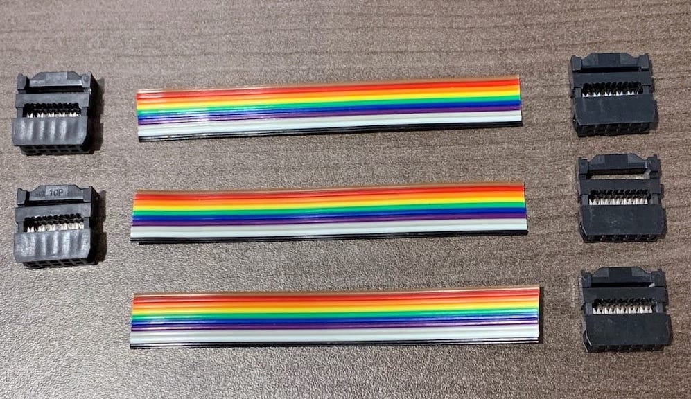
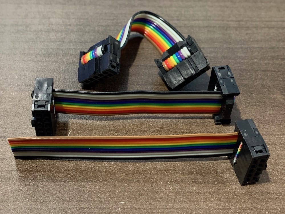
Fig 7.2-1. Components needed to assemble the 10-wire ribbon cables
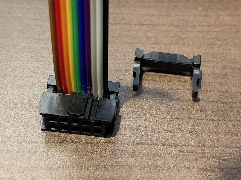
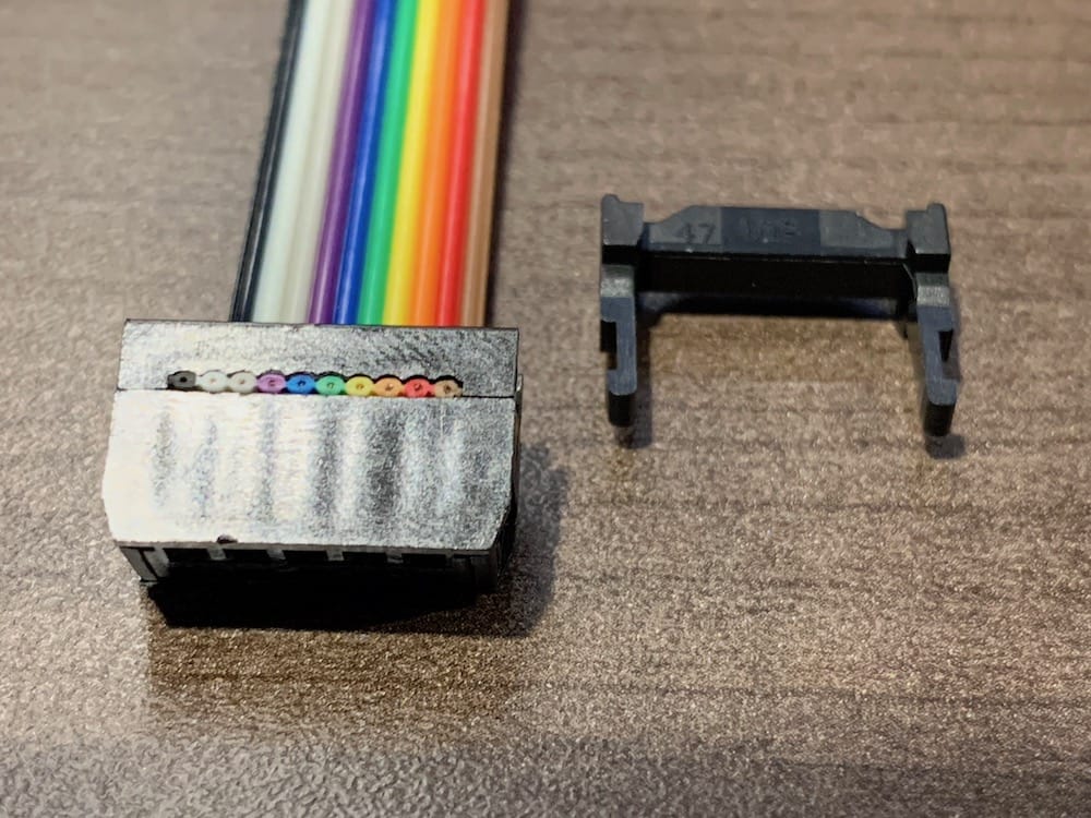
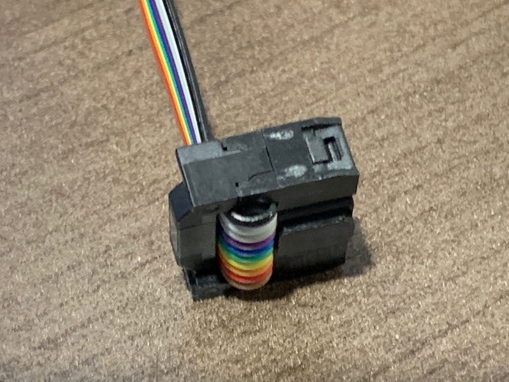
Each connector is attached to the ribbon cable in the same way. Start by removing the locking bar from the top of the connector. Find the face of the connector that has the orientation tab on it. Insert the ribbon cable into the connector going through the face with the orientation tab first. If your ribbon cable has multiple colors of wires, pay close attention to the wires’ order as each connector must have the same order of colored wires. Position the cable, so it is flush with the opposite face of the connector and crimp the connector closed. Lastly, flip the cable over the top of the connector and secure the locking bar into the connector. Repeat these instructions for all five connectors on the three cables.
7.3. Ethernet Cables
A total of four ethernet cables need to be assembled. Three of the cables are standard straight-through ethernet cables with RJ45 connectors on both ends. Due to the tight fit of these cables inside the case, the RJ45 connectors need to be modified. The remaining cable has an RJ45 connector on one end only, while the other end is directly soldered to the respective RJ45 jack on the Left Face of the case (see the Left Face Assembly section for the details).
The following components are needed to assemble the four ethernet cables.
2 @ Cat5/6 ethernet cable, 12cm in length
1 @ Cat5/6 ethernet cable, 10cm in length
1 @ Cat5/6 ethernet cable, 8cm in length
7 @ RJ45 crimp connectors
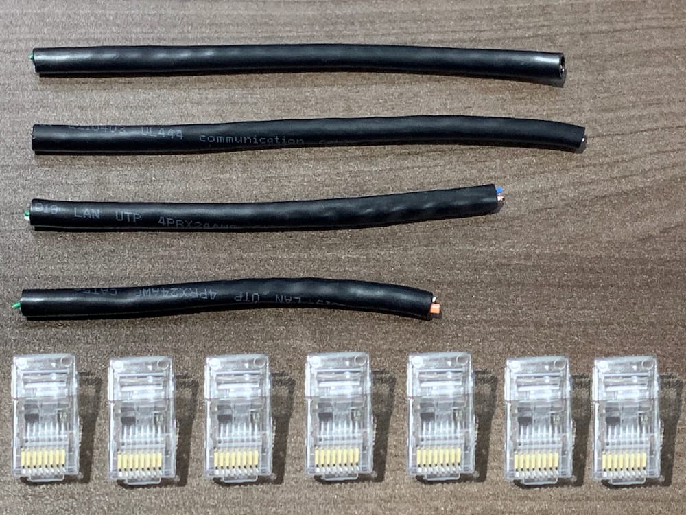
Fig 7.3-1. Components needed to assemble the ethernet cables
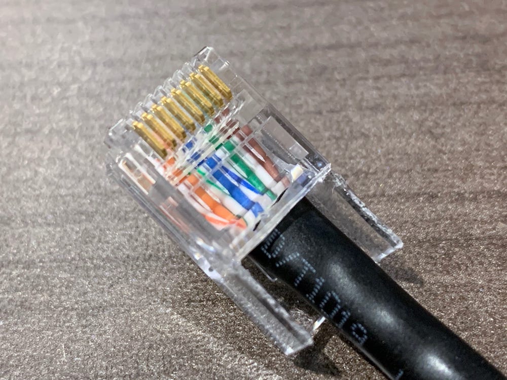
Four of the RJ45 connectors need to be modified by trimming away one side of the crimping collar opposite the side of the connector with the latching clip. Trimming the connectors is necessary to allow the ethernet cables to be bent inside the case. Start by cutting along the outside edges of the side to be removed. Next, grab the side with small pliers and bend it back and forth. Eventually, the side will come free and should leave a clean ‘cut’ where the side was connected.
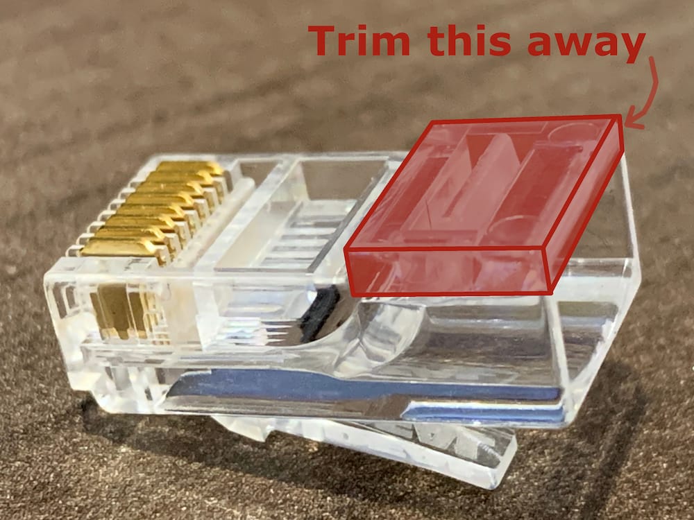
Fig 7.3-2. RJ45 side to remove
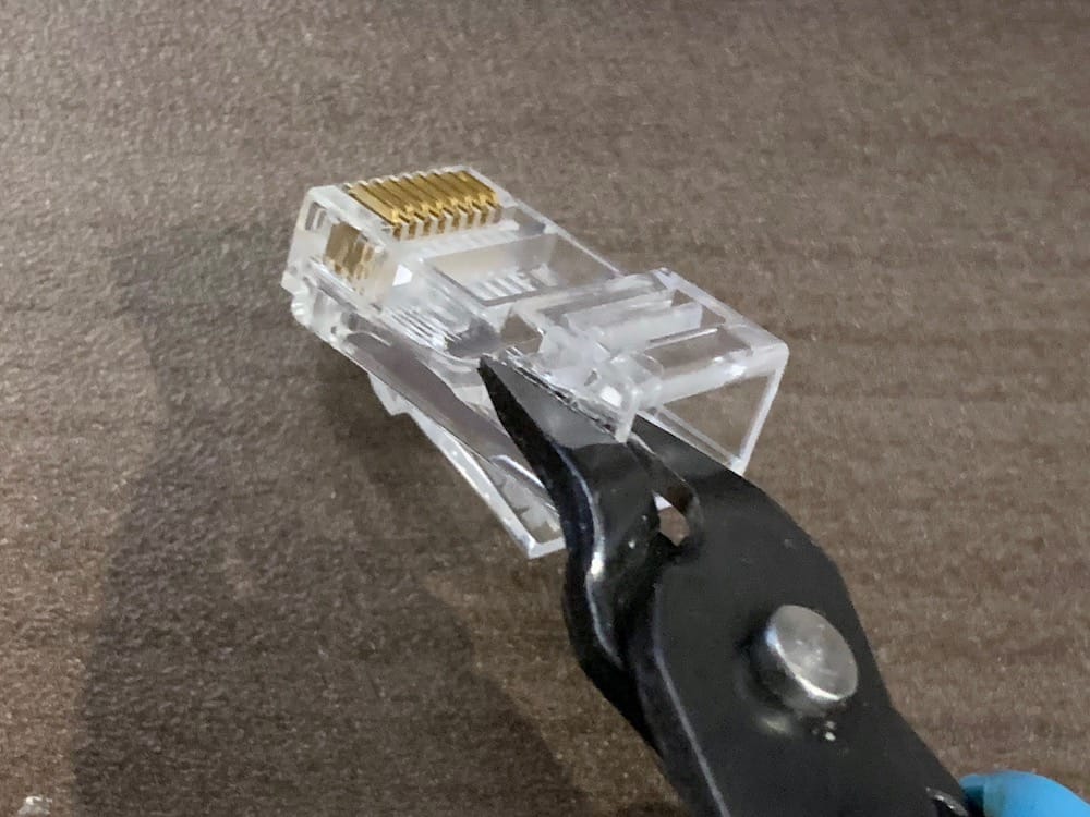
Fig 7.3-3. Cut the outside edges
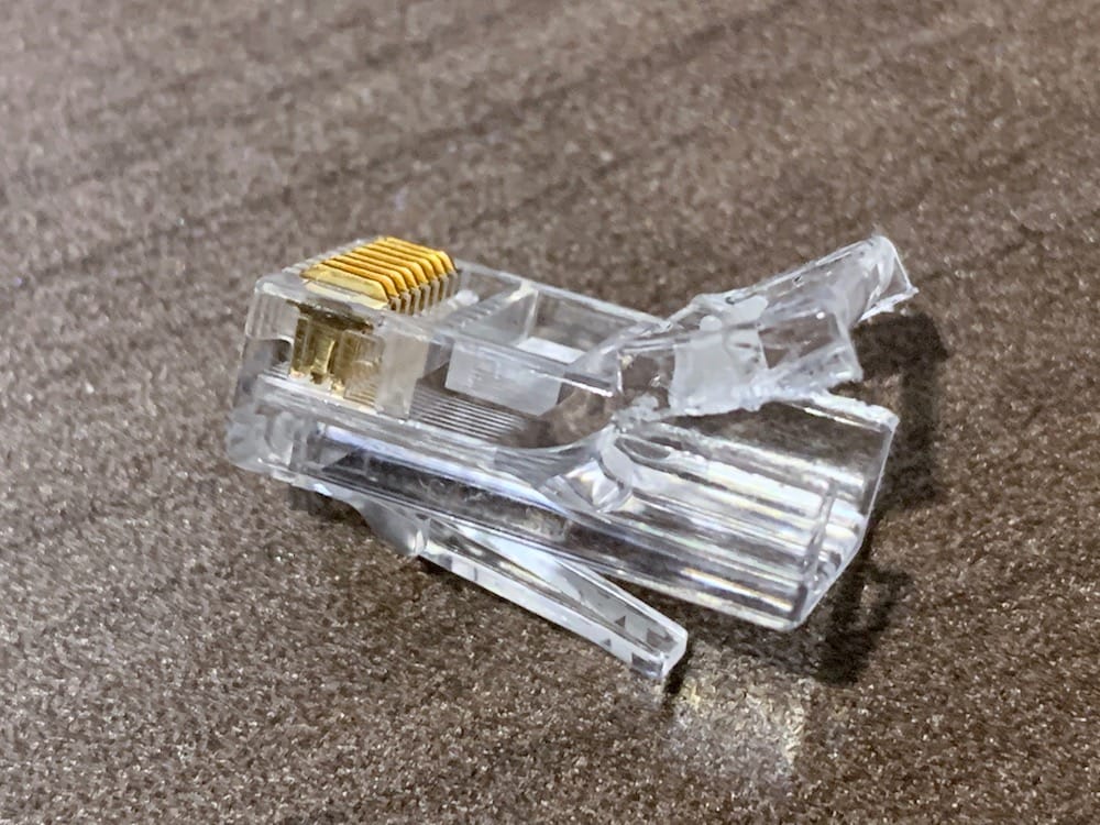
Fig 7.3-4. Bend side up and down
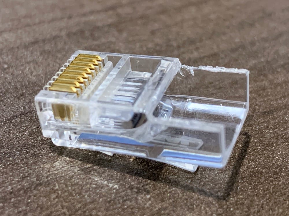
Fig 7.3-5. Modified connector A
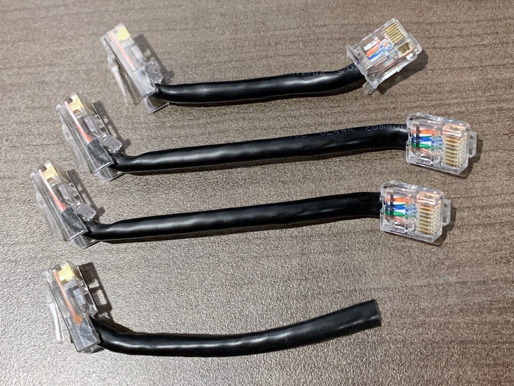
The remaining three RJ45 connectors also need to be modified by trimming away the entire crimping collar. Trimming the connector is necessary to allow the ethernet cables to be inserted into their respective components and be allowed to bend inside the case. Start by performing the same modification, as described above. Next, make vertical cuts along the edges and then bend the edges so they are flat and in line with the crimping collar’s remaining side. Next, make small cuts across the flattened corner where the edge meets the remaining side. Lastly, grab the flattened side with small pliers and bend it back and forth. Eventually, the side will come free and should leave a clean ‘cut’ where the side was connected.
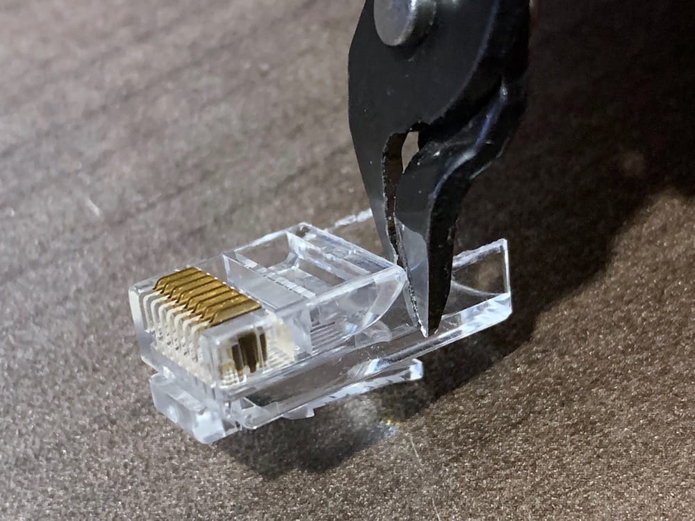
Fig 7.3-6. Vertical edge cuts
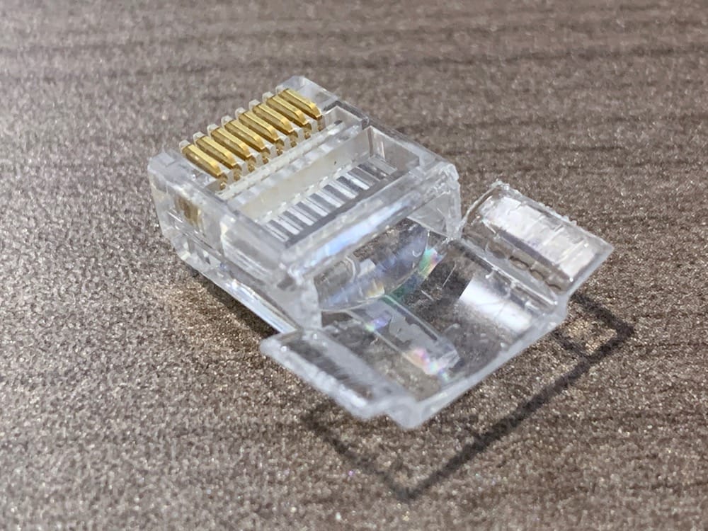
Fig 7.3-7. Flatten the edges
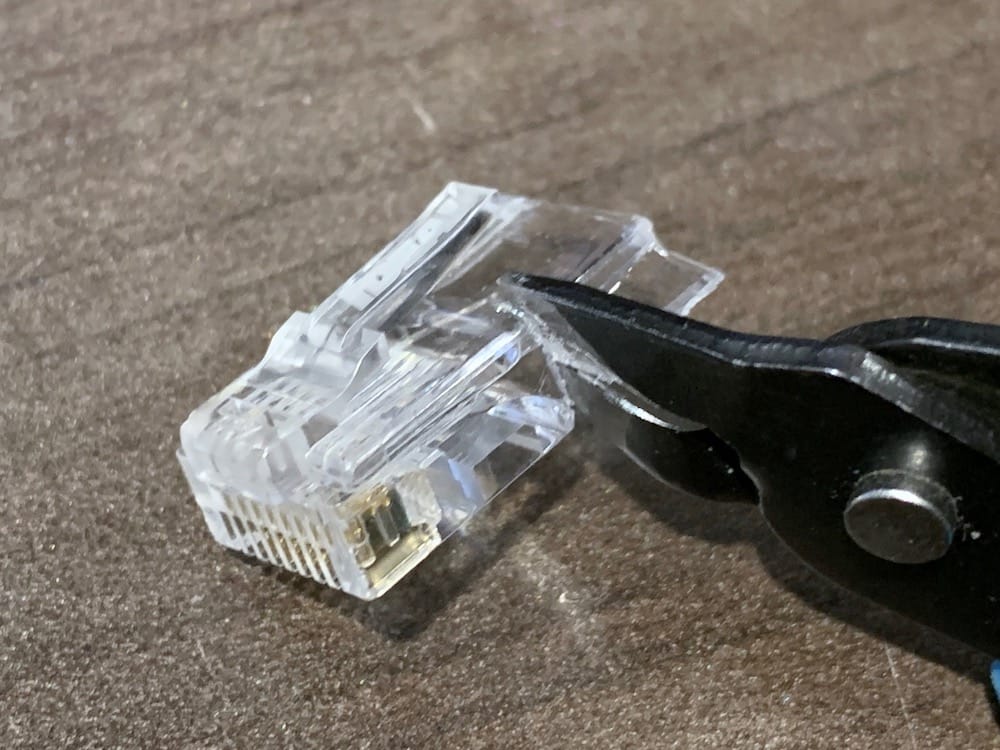
Fig 7.3-8. Snip the edge corners
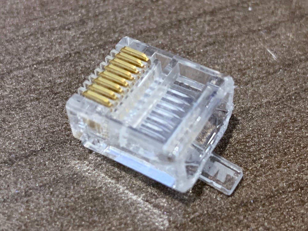
Fig 7.3-9. Modified connector B
Watch this video for information on how to properly use an RJ45 crimping tool. The OpenMMS ethernet cables follow the RJ45 T-568B connection standard, which defines the order of the eight colored wires inside each connector. The following figure illustrates the T-568B standard.
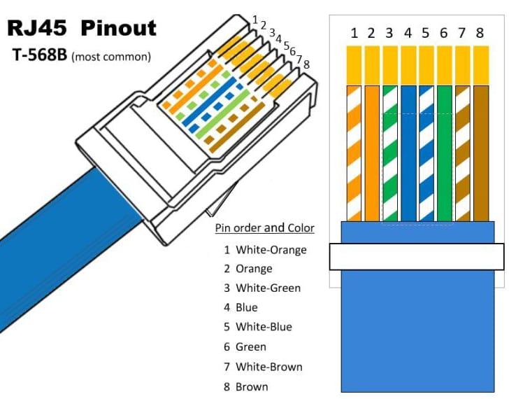
Fig 7.3-10. RJ45 T-568B connection standard
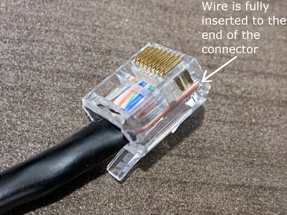
Each of the four ethernet cables has a modified connector A crimped to one end. The two 12cm long cables and the 8cm long cable, have a modified connector B crimped to the other end. Therefore, the 10cm long cable only has a connector on one end. Be sure the individual wires are in the correct order, following the T-568B standard, and fully inserted into the RJ45 connector before crimping the connector. It is practically impossible to undo a crimped RJ45 connector to fix a mistake, so be sure the wires are correct before committing to the crimp.
7.4. Sony Battery Cable
The OpenMMS sensor is designed to provide power to the Sony A6000 high-resolution RGB imagery camera. To do this, a ‘dummy’ battery is used in place of the original Sony battery. The dummy battery has a cable attached to it, which runs external to the camera and plugs into the Left Face of the OpenMMS case via a 2-pin Lemo connector. Unfortunately, the Sony batteries for the A6000 camera do not only provide a positive voltage connection and a ground connection to the camera. There is a 3rd connection that transfers data between the camera and the battery. Because of this fact, the dummy battery must transfer the necessary data between itself and the camera. Thankfully ‘smart’ dummy batteries are commercially available and are required for making the OpenMMS Sony Battery Cable. An original Sony A6000 battery can be used instead of the OpenMMS Sony battery cable if desired. However, the user needs to ensure the battery is adequately charged before the OpenMMS sensor is used.
The following components are needed to assemble the Sony Battery Cable.
1 @ Smart Dummy Battery replacement for the NP-FW50 battery
1 @ 2 pin Lemo 0B series connector
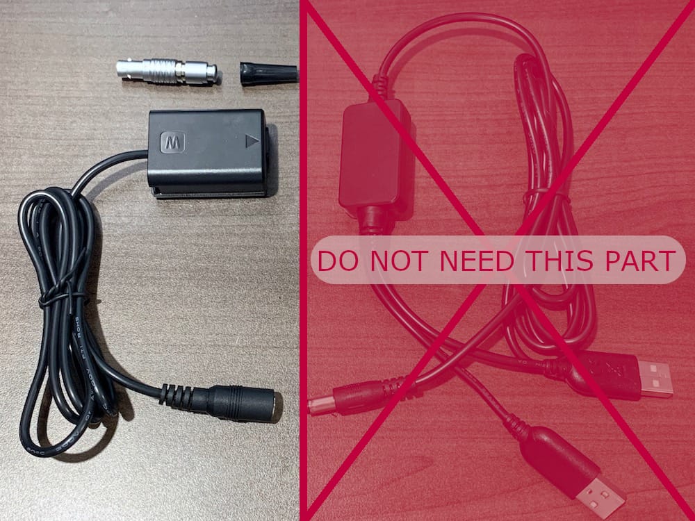
Fig 7.4-1. Components needed to assemble the Sony Battery Cable
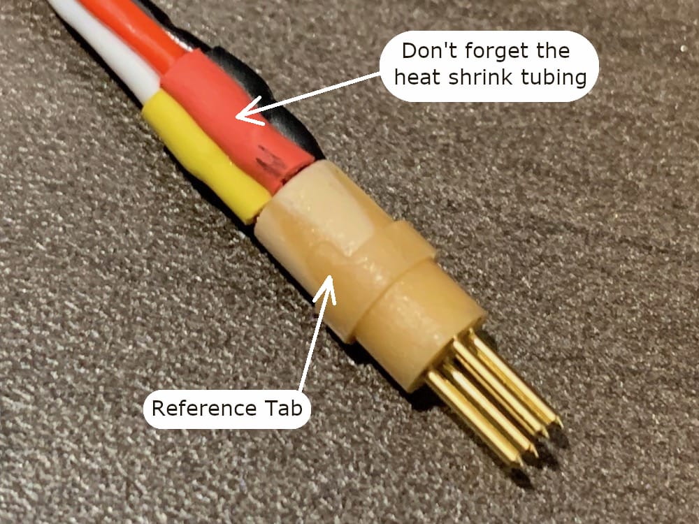
Start by cutting the cable coming out of the dummy battery to a length of 12cm and disassembling the 2-pin Lemo connector components. Next, carefully strip about 15mm of the sheathing at the cut end of the battery cable, and expose the red positive voltage and black ground wires. Strip a few millimeters of sheathing from each of the wires and then ‘tin the tip’ of each wire using a soldering iron and melting a small amount of solder onto and throughout the exposed wires. Tinning the tips makes soldering the wires to the small Lemo connector pins much easier. Next, slide the Lemo connector components - IN THE CORRECT ORDER - onto the battery cable. It is recommended to include a small piece of heat shrink tubing on the cable before the Lemo components. Cut small pieces of heat shrink tubing and place them over each of the wires. Next, solder the red positive voltage wire to the top Lemo pin. The top pin is defined as the pin that is closest to the reference tab on the Lemo pin housing. Solder the black ground wire to the bottom Lemo pin.
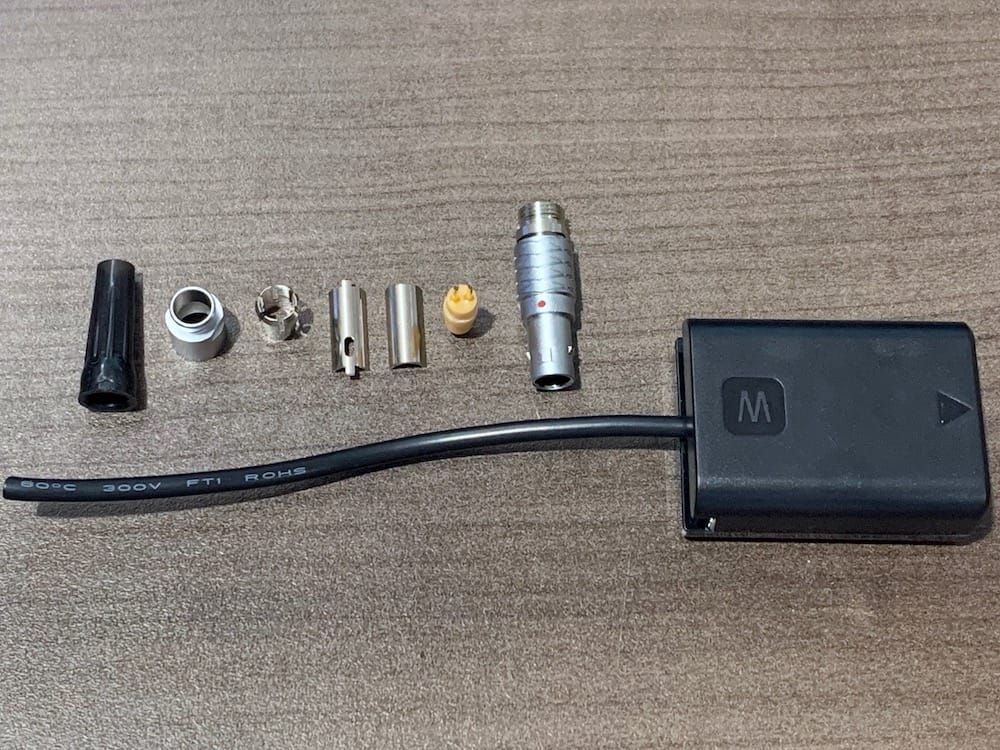
Fig 7.4-2. Cable cut to length
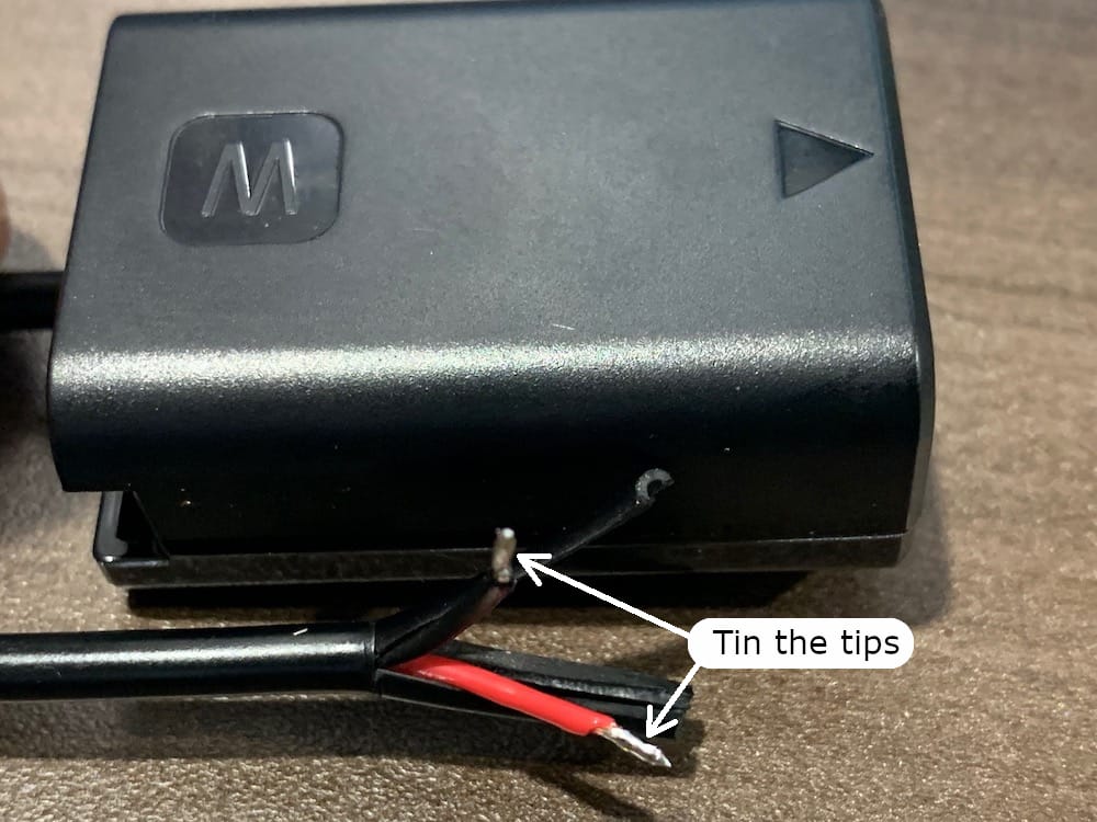
Fig 7.4-3. Cable and wires stripped
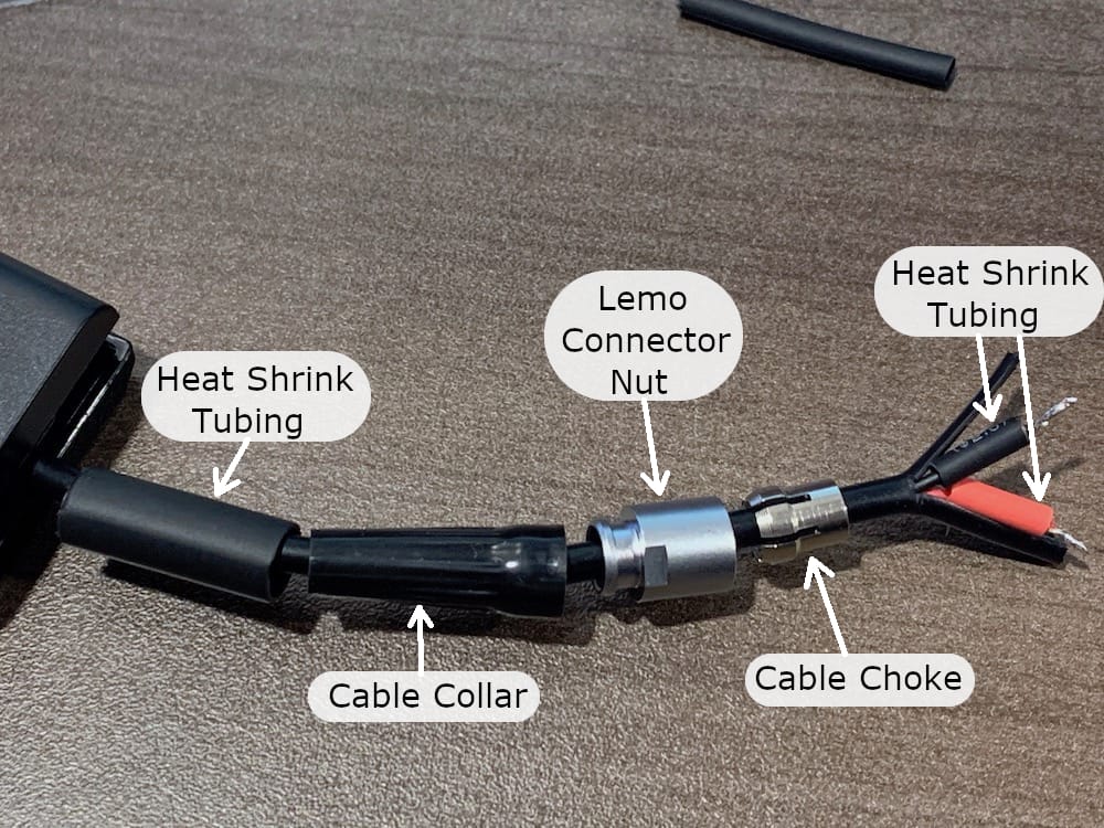
Fig 7.4-4. Ordered Lemo components
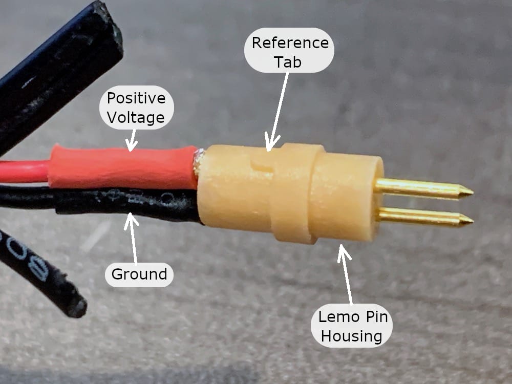
Fig 7.4-5. Lemo pin housing
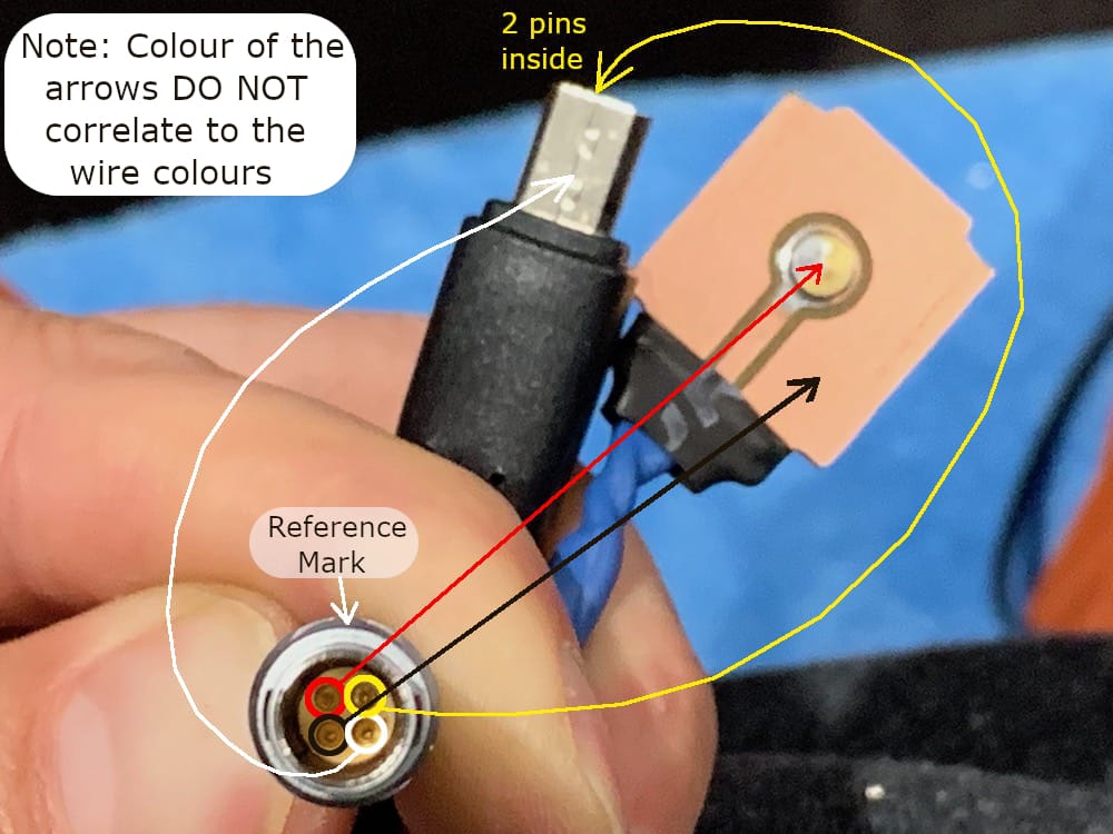
Next, install the two halves of the Lemo cable guide around the pin housing. Pay close attention to the machined grooves on the insides of the two halves of the cable guide. The guide can only be properly installed one way. The halves need to be held in place by hand. Next, insert the pin housing and cable guide into the Lemo connector. The notch on the top half of the cable guide needs to be in line with the Lemo connector’s reference dot. An excellent way to ensure they are aligned is to purposely misalign the notch on the top while inserting the pin housing into the connector. Then slowly rotate the pin housing while applying forward pressure on the cable. You should feel the cable move farther into the connector when the correct alignment is realized. While keeping forward pressure on the cable within the Lemo connector, slide the cable choke, followed by the Lemo connector nut, up the cable and into the backside of the connector. Thread the Lemo connector nut onto the threads on the backside of the connector and tighten. The nut and connector both have flat sides where a small wrench or pliers can be used to tighten the nut firmly. Next, slide the cable collar up the cable and force it onto the Lemo connector nut’s locking edge.
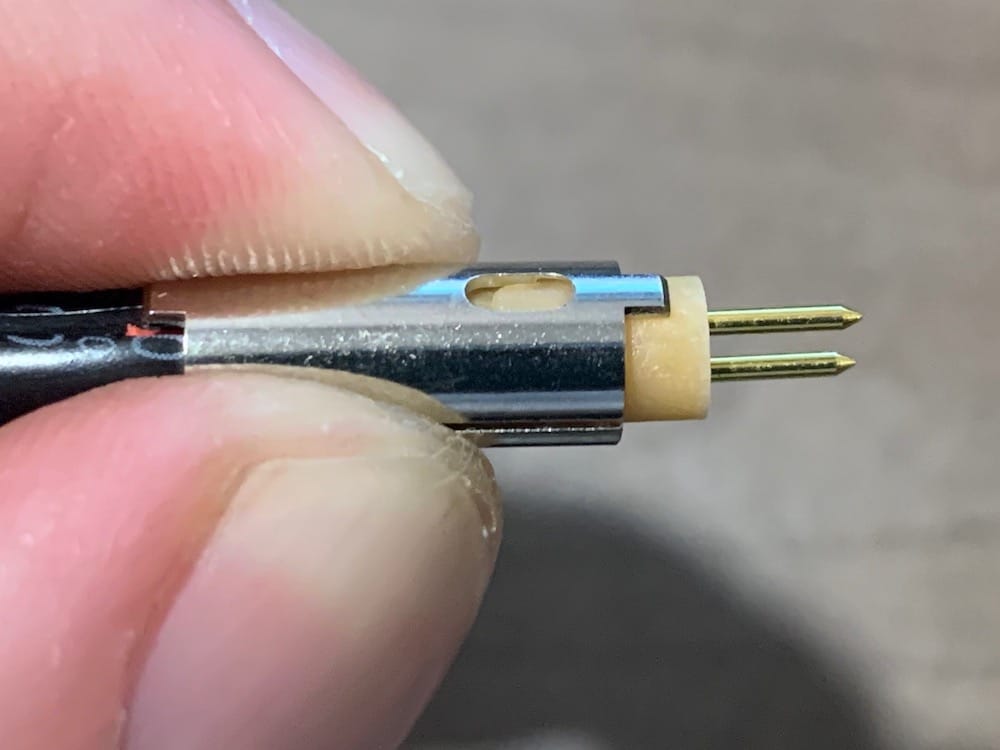
Fig 7.4-6. Lemo cable guide
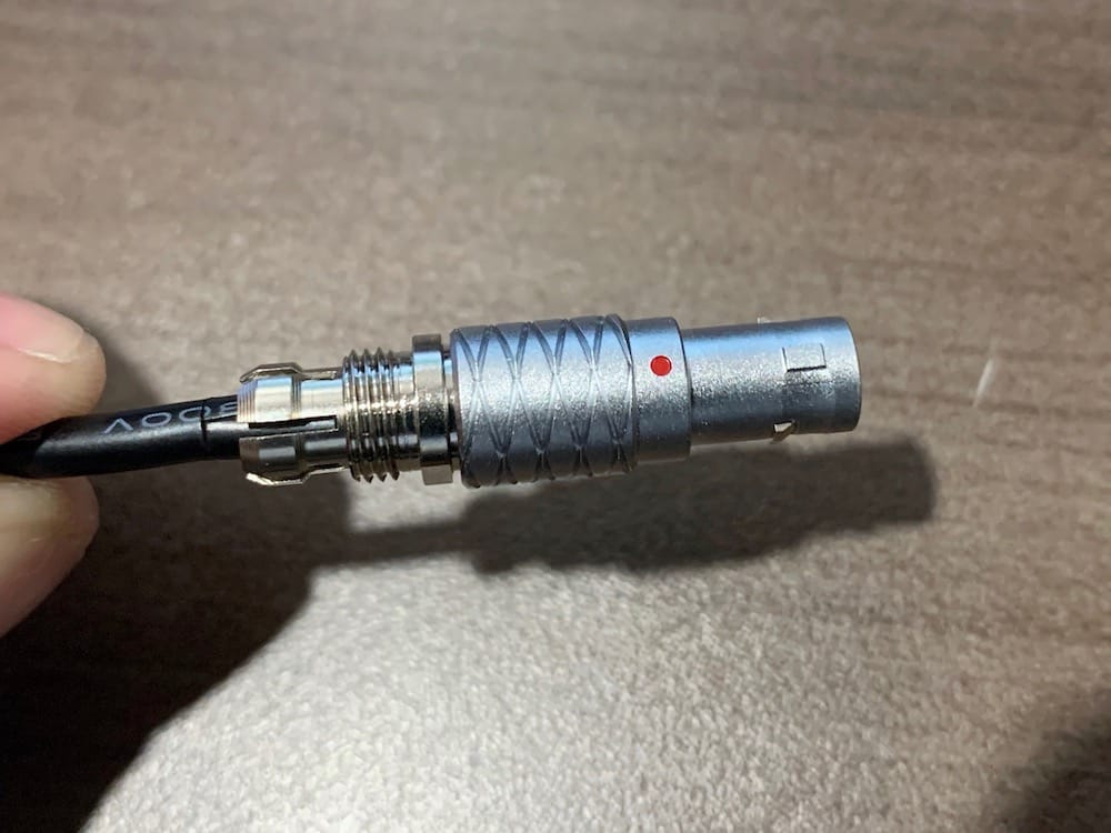
Fig 7.4-7. Cable choke in place
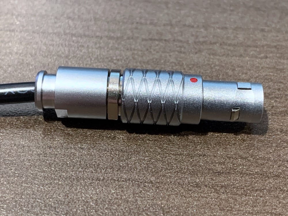
Fig 7.4-8. Lemo connector nut
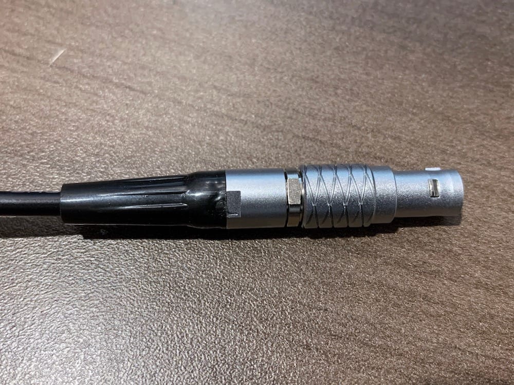
Fig 7.4-9. Cable collar in place
Lastly, if utilized, slide the heat shrink tubing up the cable and have it adequately cover a portion of the cable collar and a portion of the cable itself. Apply heat to set the tubing in place.
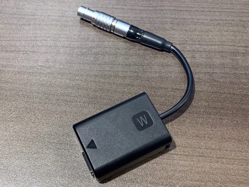
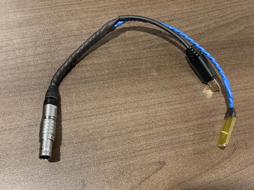
Fig 7.4-10. Completed OpenMMS Sony battery cable
7.5. Sony Trigger and Event Cable
The OpenMMS sensor is designed to control when the Sony A6000 camera takes a photo, based on a user-specified time interval (currently the only available option). However, it takes the Sony A6000 camera a variable amount of time after receiving the command, before it takes the photo. It is also possible that the camera may not take a photo even though it received the command. To capture the precise time each photo was taken, a sensor is installed in the Sony A6000’s external flash ‘hot-shoe’ connector. The camera sends a signal to the flash connector at the precise time when the camera’s shutter is opened. The sensor captures this signal and, after being conditioned, sends it to the Applanix APX-18 GNSS-INS sensor, where the precise timing is recorded as an Event. A single cable needs to be created that provides both the camera triggering functionality and capturing when a photo Event occurs.
The following components are needed to assemble the Sony Trigger and Event Cable.
1 @ TuffWing - Hot-shoe precision geotag cable
1 @ Vello - Sony shutter release cable
1 @ 4 pin Lemo 0B series connector
Some extra 26 AWG flexible wire (not shown)
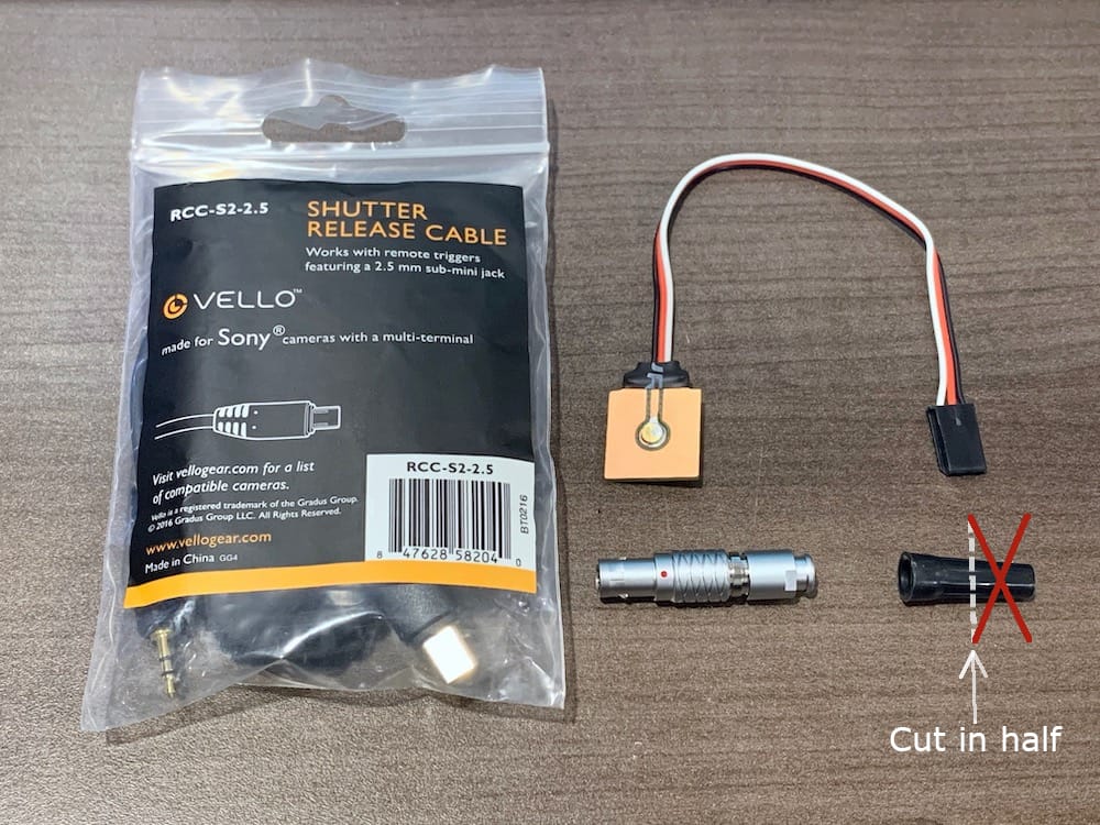
Fig 7.5-1. Components needed to assemble the Sony Trigger and Event Cable
Start by taking the Sony A6000 camera and making a reference line across the flash hot shoe connector that aligns with the silver pad near the center. Next, carefully insert the TuffWing hot-shoe precision geotag cable into the hot-shoe connector, making sure to depress the center pin with a thin, rigid object. Seat the geotag cable as far into the hot-shoe connector as possible. Compare the reference line previously made with the center pad on the backside of the geotag cable. If the geotag cable’s center pad is above the reference line, the bottom edge of the geotag cable’s PCB needs to be adjusted. If the geotag cable’s center is below the reference line, no adjustments need to be made.
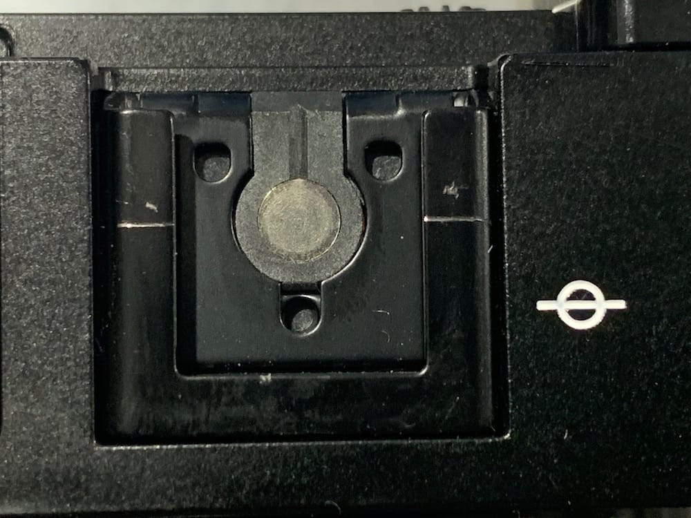
Fig 7.5-2. Reference line
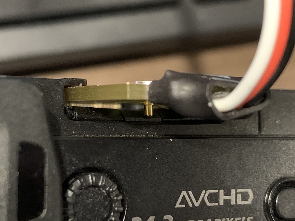
Fig 7.5-3. Geotag cable center pin
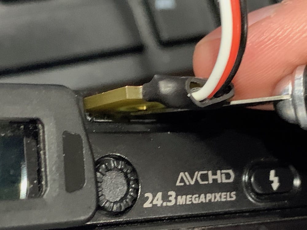
Fig 7.5-4. Center pin is depressed
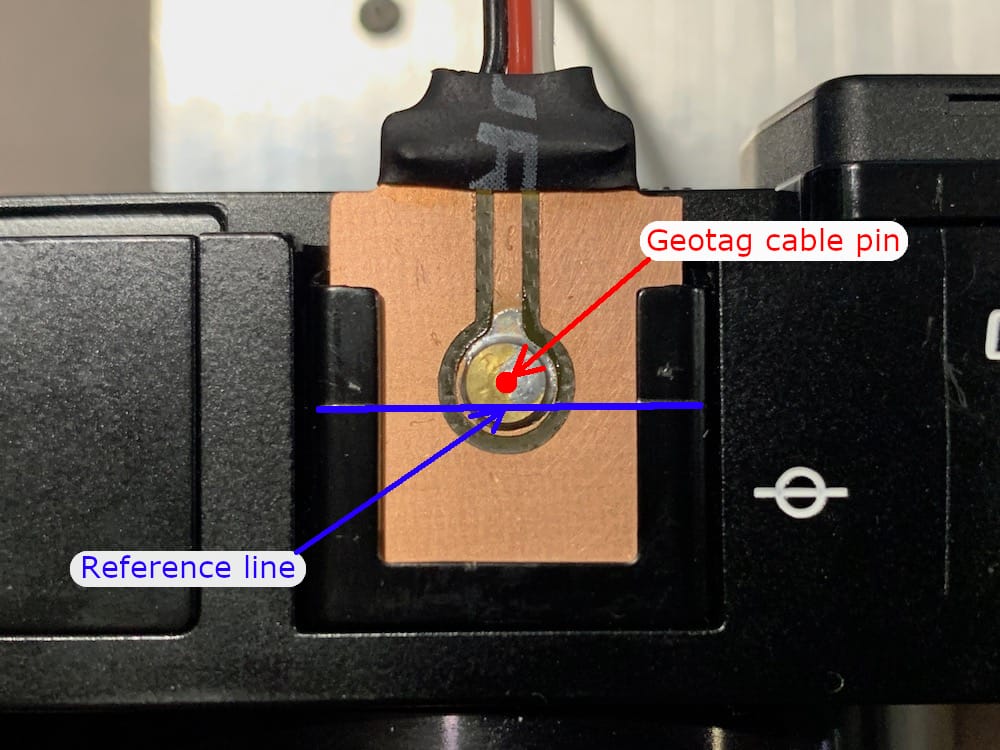
Fig 7.5-5. Initial fit in hot-shoe
If the geotag cable’s center is above the reference line, the bottom corners of the cable’s PCB should be carefully snipped away. Approximately a 3mm (left to right) by 1.5mm (top to bottom) area should be removed from each corner. The bottom edge on the PCB’s non-copper side must also be filed at a 45 deg angle to create a tapered edge. Lastly, reinsert the geotag cable into the hot shoe and observe if the adjustments have improved the center pin’s alignment with the reference line. Continue to make small adjustments until the alignment is correct. Remove the geotag cable from the camera before continuing.
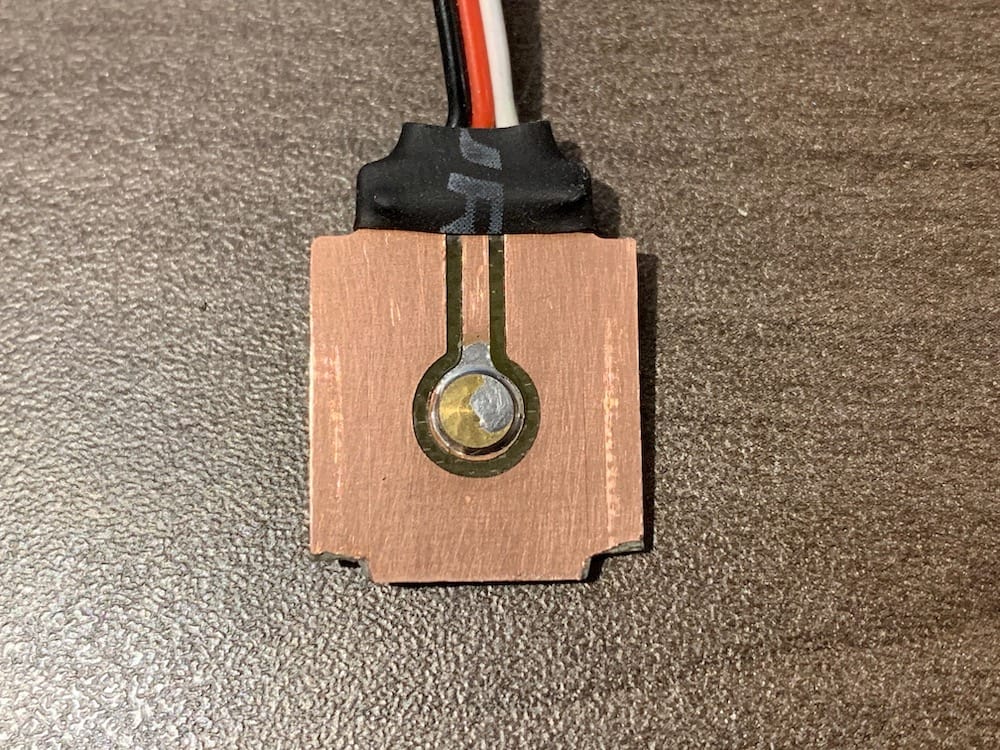
Fig 7.5-6. Adjusted bottom corners
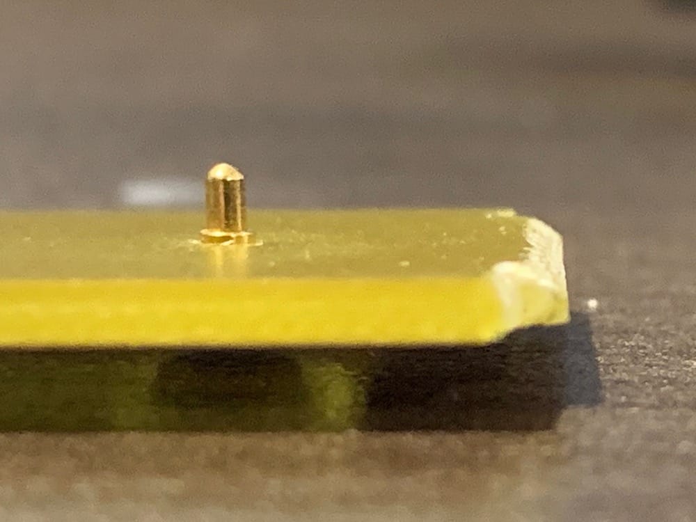
Fig 7.5-7. Tapered bottom edge
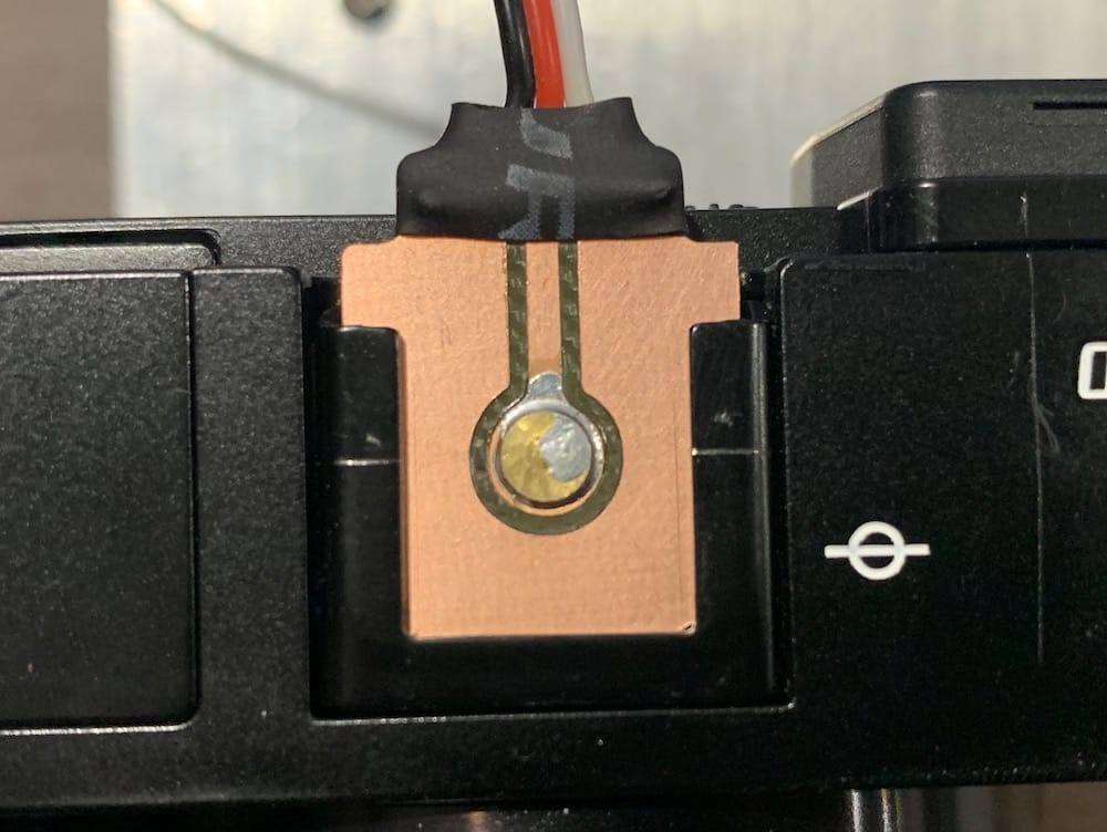
Fig 7.5-8. Correct alignment in hot shoe
Next, take the Vello shutter release (trigger) cable and cut it on the USB (multi) connector side just before the cable begins to twist. Strip the cable’s sheathing approximately 20mm from the cut end, being very careful not to damage any of the three wires inside. Expose and red, green, and blue wires and strip away 5mm of their sheathings. These wires also have pieces of nylon thread inside them. It is recommended to cut away these nylon threads to make soldering them easier and cleaner. Next, using a multimeter with a continuity tester, confirm that the blue wire is connected to the ground surface of the USB (multi) connector (it should be). If the blue wire is not connected to ground for some reason, then one of the other two wires must be. There should only be one ground wire in the cable. Next, take the two other (non-ground) wires and connect them together. Tin the tips of the joined pair of wires and the ground wire. Extend the two wires by soldering the extra 26 AWG flexible wire so the Vello release cable is approximately 17cm in length measured from the back end of the USB (multi) connector. It is strongly recommended that the ground wire be extended using a black-colored wire and the connected pair of wires be extended using a red-colored wire.
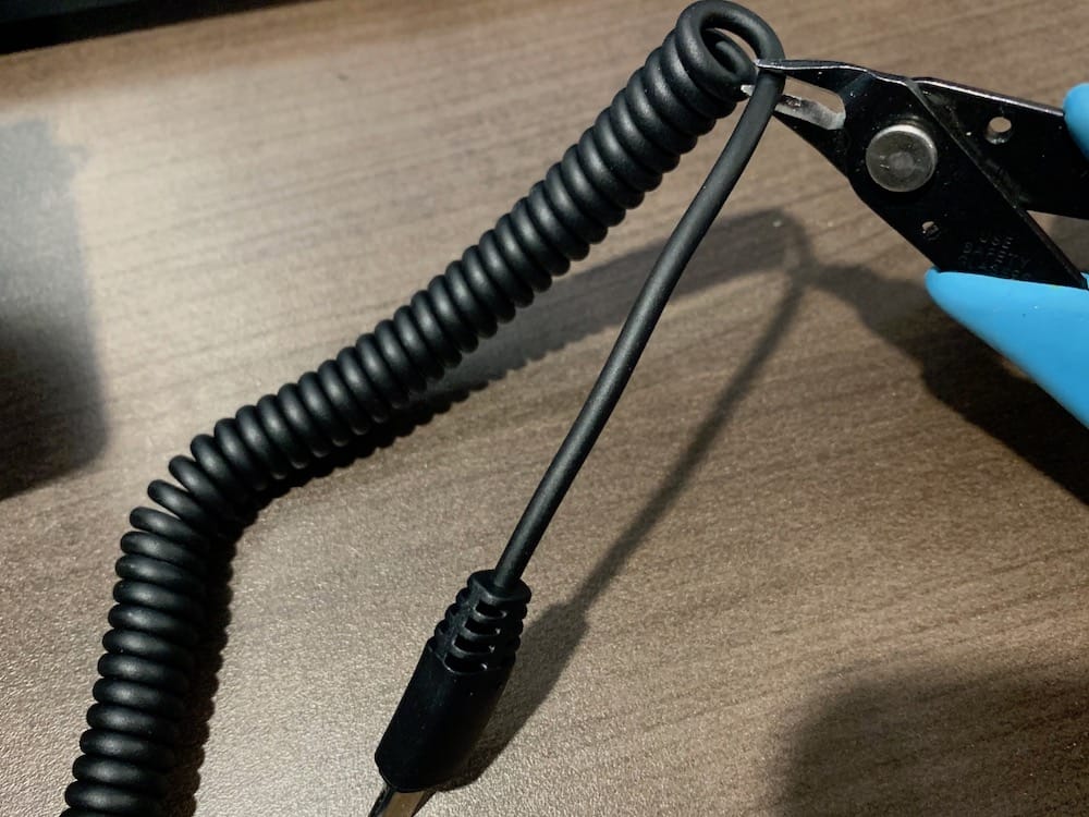
Fig 7.5-9. Cut Vello release cable here
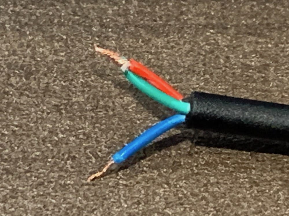
Fig 7.5-10. Ground (B), focus (G), shutter (R)
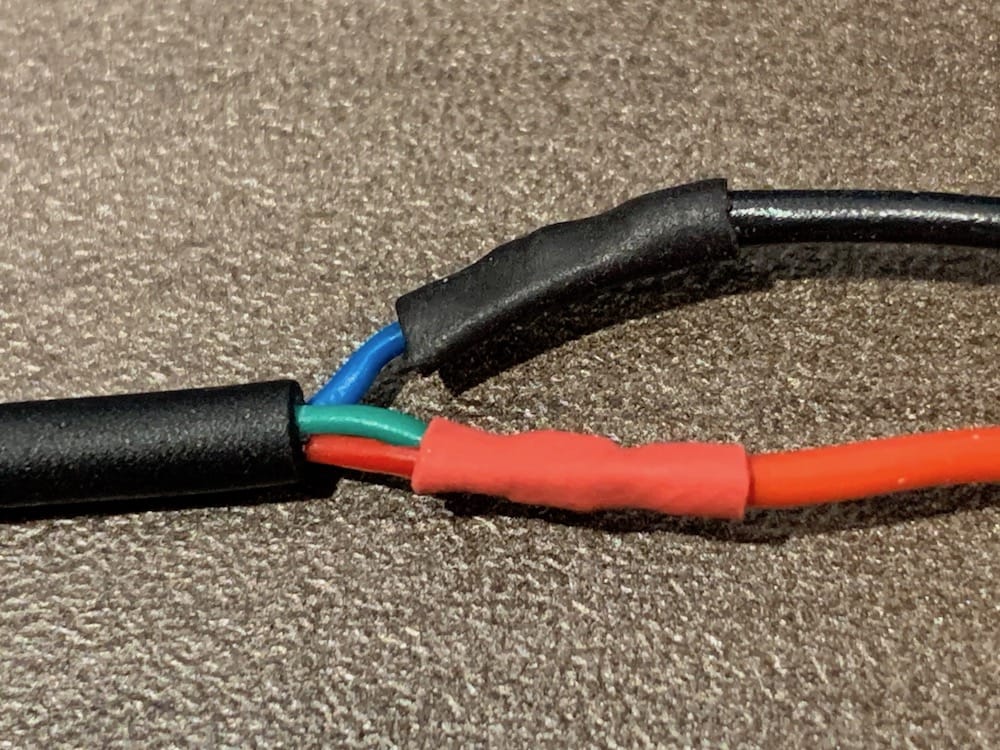
Fig 7.5-11. Focus & shutter connected together
Next, cut and discard the JR connector end from the TuffWing hot-shoe precision geotag cable. Remove the center (red) wire from the three wires, as it is not connected to the PCB and, therefore, not needed. Strip away 5mm of sheathing from the remaining two wires and extend them by soldering the extra 26 AWG flexible wire, so the TuffWing geotag cable is approximately 20cm in length measured from the back end of the PCB connector. It is strongly recommended that the geotag cable wires be extended using wires of the same color (e.g., white and black shown here). Next, apply heat shrink tubing individually to the entire length of the extended Vello release cable and the TuffWing geotag cable. Apply an additional 8cm length of heat shrink tubing around BOTH cables to join them together. Ensure 2-3cm of the exposed individual wires is outside the additional heat shrink tubing to allow for the individual wires to be soldered to the Lemo connector.
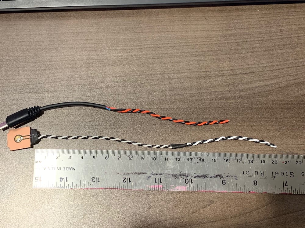
Fig 7.5-12. Extended cable lengths
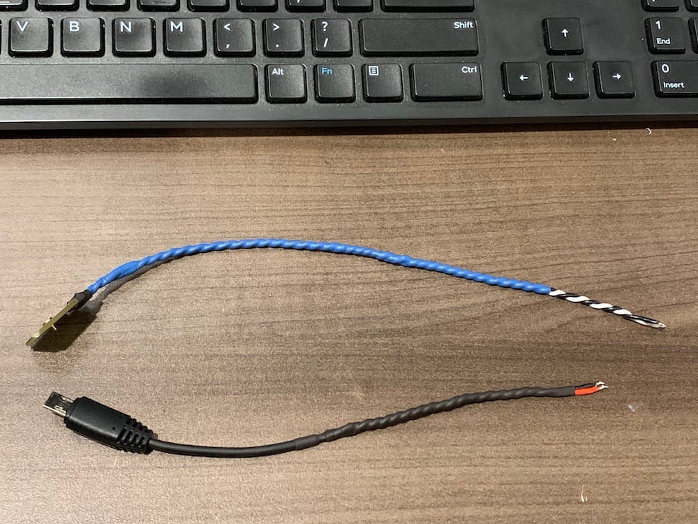
Fig 7.5-13. Heat shrink tubing around each cable
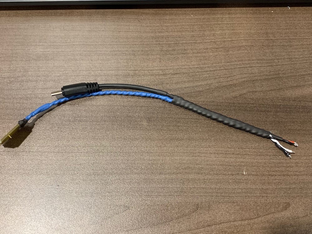
Fig 7.5-14. Additional heat shrink to join the cables
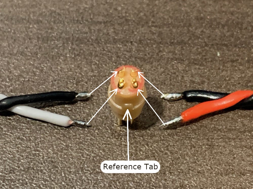
Next, disassemble the 4-pin Lemo connector and slide the respective components (IN THE CORRECT ORDER) onto the cable (see Sony Battery Cable section for Lemo connector details). It is recommended to cut the black Lemo cable collar approximately in half to allow for better cable flexibility. Include a piece of heat shrink tubing as the first component to slide onto the cable. Solder the four wires to the respective pin connectors on the backside of the Lemo pin housing, as shown in the figure below. Use heat shrink tubing around each soldered wire to insulate them from each other and the Lemo connector housing. Remember the black wires are ground wires, the red wire is the trigger wire, and the white wire is the Event wire, within this example. AFTER SOLDERING, IT IS STRONGLY RECOMMENDED TO TEST FOR SHORT CIRCUITS ACROSS ALL FOUR PINS TO ENSURE NONE EXIST! Next, slide the Lemo components pre-installed on the cable to the Lemo connector to complete the cable assembly. Check for continuity between the Lemo pins and the Vello and TuffWing connectors on the cable, as shown in the figure below.
7.6. GNSS Antenna Cables
Attention
The following instructions will create GNSS antenna cables with the proper end connectors for connecting the Applanix APX-18 GNSS-INS sensor to Trimble AV14 GNSS antennas. If different GNSS antennas are utilized, it is the reader’s responsibility to ensure that suitable GNSS antenna cables are used.
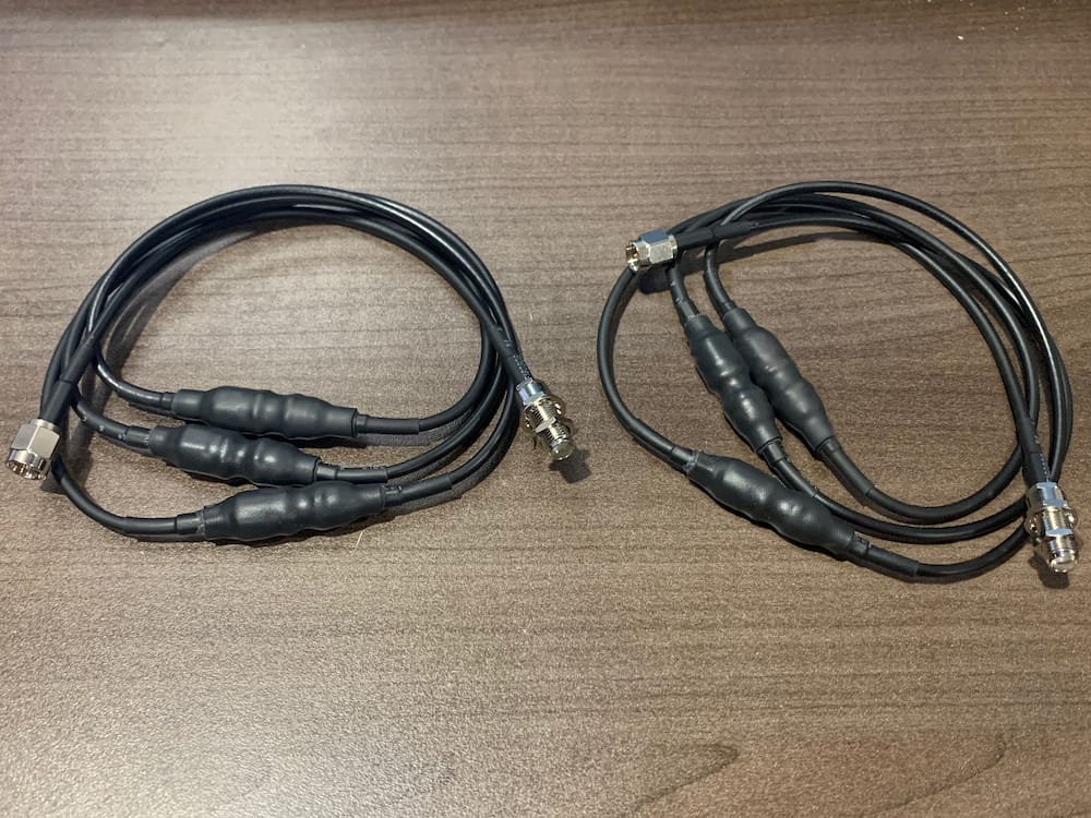
A total of two GNSS antenna cables need to be assembled. Cables that are directly ready to use could be purchased from other sources than those listed in the Getting Started –> List of Sensors and Electronics section. An interested reader could explore the Classic Builder tool on www.onlinecables.com. The GNSS antenna cables need to have an SMA male connector (straight or right-angle) on one end, a 50 Ohm shielded coaxial cable (e.g., RG-174), a straight SMA female connector on the other end, and be 100cm in length.
The following components are needed to assemble the two GNSS antenna cables using the parts listed in the Getting Started section.
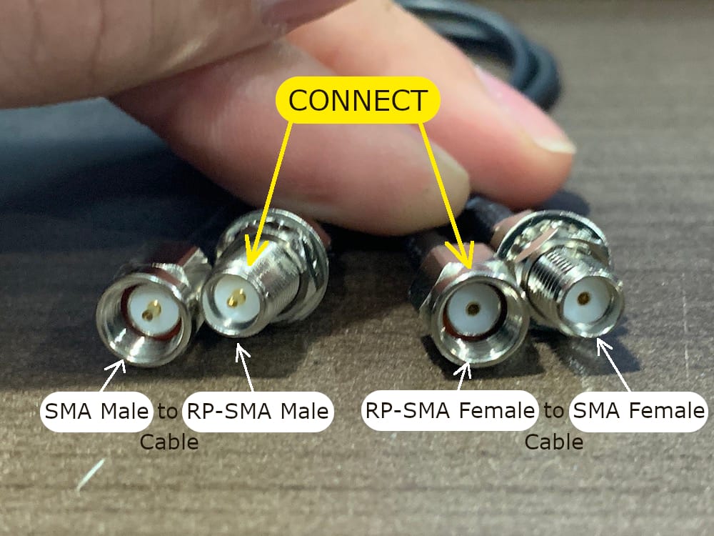
4 @ SMA Male to RP-SMA Male coaxial cable, 25cm in length each
4 @ RP-SMA Female to SMA Female coaxial cable, 25cm in length each
Heat-shrink tubing
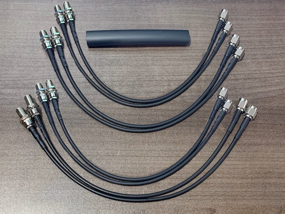
Fig 7.6-1. Components needed to assemble the GNSS antenna cables
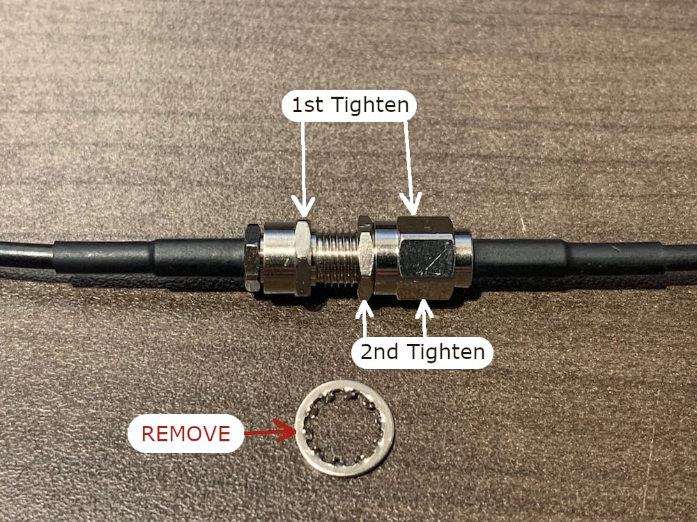
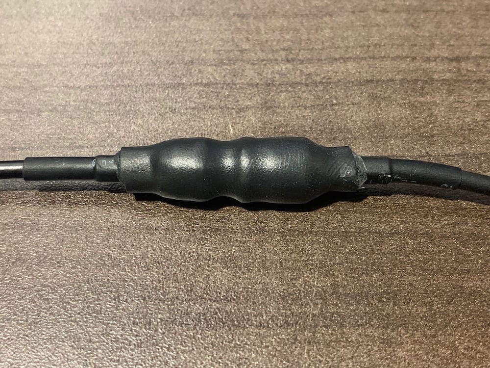
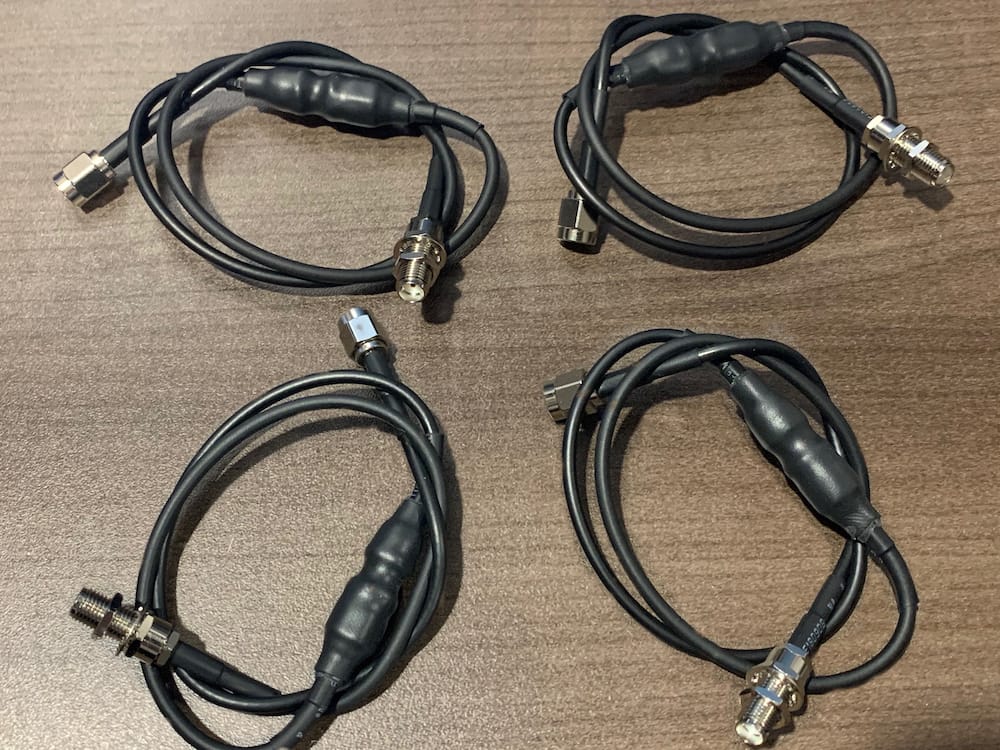
If the listed coaxial cables are used, the first step is to connect one of the SMA Male to RP-SMA Male cables with one of the RP-SMA Female to SMA Female cables. Please pay close attention that the right ends of each cable are connected, as it is possible to connect the wrong ends, see the figure below. The star washer should be removed where the cables connect as it does not provide any benefit to the connection. However, the nut needs to be used, so ensure it is put back onto the connector after removing the star washer. Tighten the connectors together first, and then tighten the nut. Apply an adequate size piece of heat-shrink tubing over the connection and set it in place with a heat gun. Repeat this assembly step four times, creating four ~ 50cm length coaxial cables with the necessary SMA male and SMA female connectors. Lastly, to create the correct length of coaxial cables, two ~50cm length cables are connected following the previous instructions. Ensure to leave the star washer on the SMA female connector of the final cables as it will be used when attaching the cables to the carbon fiber GNSS antenna arms.
CONGRATULATIONS!
YOU HAVE NOW FINISHED ASSEMBLING ALL OF THE CABLES!
8. Component Configurations
8.1. Overview
There are six OpenMMS components that need to be individually configured before being installed within the OpenMMS sensor. Some of the following configuration instructions require the reader to possess certain computer networking skills (e.g., DHCP vs. static IP address assignment). When possible, links to helpful articles/videos are provided to help the reader acquire the necessary skills. Detailed explanations of these skills are not provided within the OpenMMS documentation.
8.2. Matek Systems UBEC Duo
The UBEC Duo serves as the primary voltage regulator for the OpenMMS sensor. It supports unregulated input voltages between 12V (OpenMMS minimum) and 26V (i.e., 4-6S LiPo batteries). It provides two regulated output voltages, the first (OUT-1) is configurable and can to set to 5V, 6V, 7.2V, or 12V, and the second (OUT-2) is fixed at 5V. Both outputs provide a maximum current of 4A, which is more than enough for the OpenMMS sensor.
For the OpenMMS sensor, the OUT-1 voltage needs to be configured to be 12V. Optionally, the UBEC Duo’s low voltage alarm values can also be configured, which can come in very handy if powering the OpenMMS sensor using a small battery. The voltage alarm can also be turned off is desired; by default, the alarm is on.
Before configuring the UBEC Duo, it is required to shorten the input and output wires. The input wires are ~20cm in length and do not have an end connector attached to them (DC IN). Shorten these wires to be ~12cm in length and solder a male 2-wire JST connector to the end (as always, be sure to use heat-shrink tubing to insulate the soldered connections). Next, the two sets of output wires are ~30cm in length and have a 2-wire JST connector on OUT-1 and a 2-wire JR connector on OUT-2. Shorten both of the output wires also to be ~12cm in length, but be sure to reconnect the original connectors to the respective wires (BE CAREFUL TO MAKE SURE THE POLARITY OF THE WIRES IS CORRECT).
Lastly, follow the instructions provided by Matek Systems (shown in the figure below), configure the OUT-1 voltage to 12V, and optionally configure the low voltage alarm to the desired setting. The UBEC Duo’s input will need to be connected to an adequate power supply to perform the configuration.
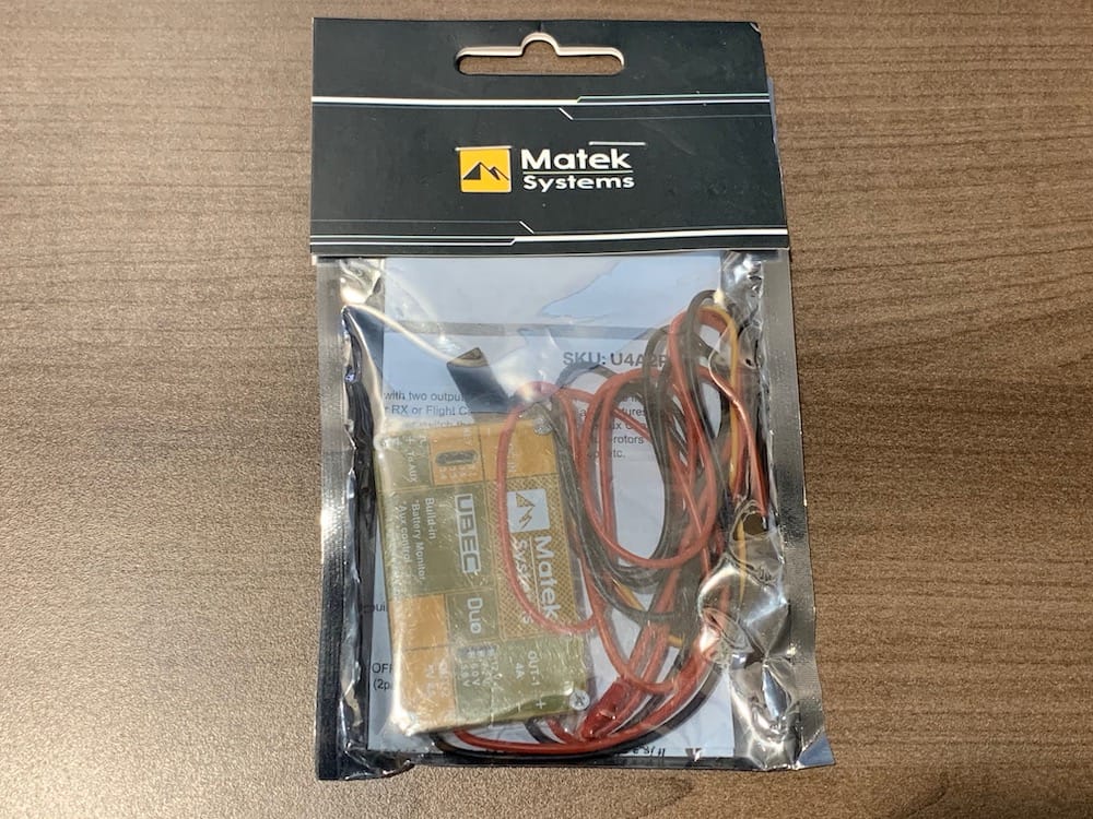
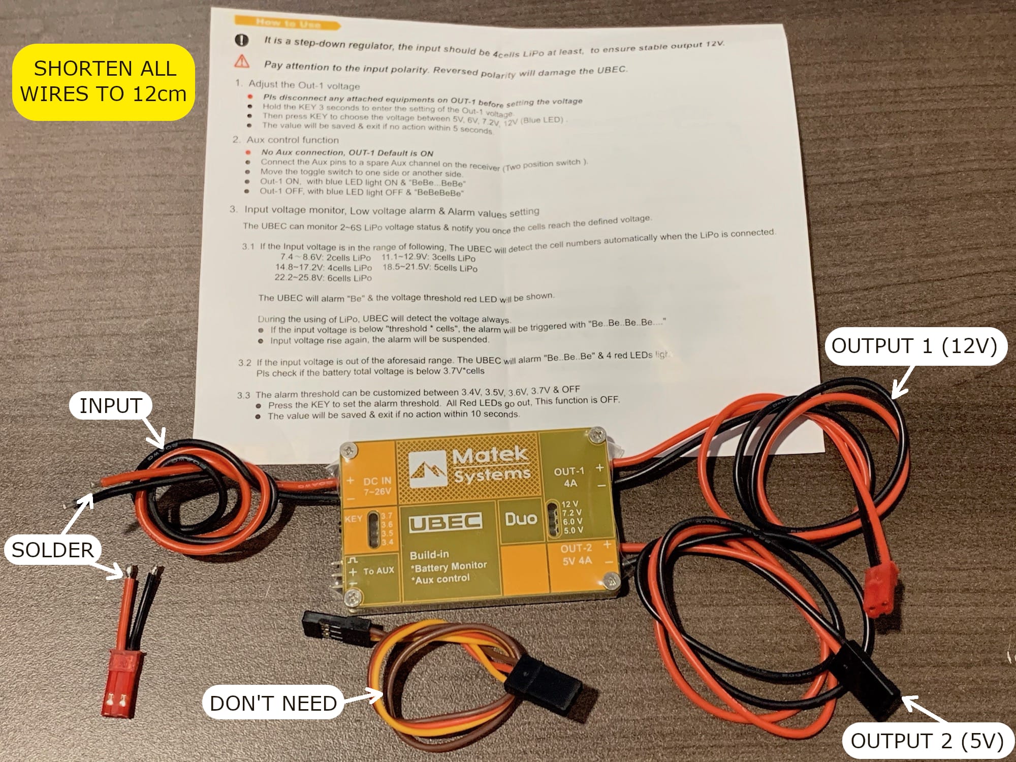
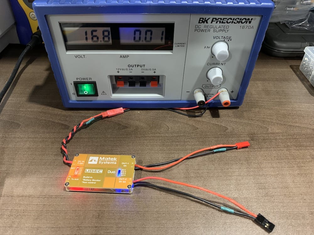
8.3. Adafruit Pro Trinket (3V)
The Adafruit Pro Trinket is a derivative product of the amazing Arduino open-source hardware project. The 3V version of the device was used to match the logic levels of a Raspberry Pi computer. The Trinket is used as a software-defined intervalometer for controlling when the Sony A6000 camera takes a photo. Before starting data collection, one of seven different time intervals can be set and changed dynamically by the field operator of an OpenMMS sensor. The time intervals are 1.5s, 2.0s, 2.5s, 3.0s, 3.5s, 4.0s, 5.0s. The Raspberry Pi computer sends three digital (LOW/HIGH) signals to the Trinket, which are used to provide a 3-bit number, indicating which time interval the Trinket should use. The available time intervals are hard-coded into an Arduino sketch (program), which needs to be uploaded to the Trinket. An interested reader could make changes to the sketch to utilize different time intervals if desired. However, the OpenMMS sensor has NOT been designed to allow for easily updating the Trinket’s Arduino sketch after it has been soldered on the OpenMMS RPi printed circuit board (PCB) and installed within the sensor case.
Refer to the OpenMMS Applications area in the OpenMMS Software section for the latest Intervalometer Sketch to upload to the Adafruit Pro Trinket device.
To install the sketch, the Arduino IDE software needs to be installed on the reader’s computer. For readers new to Arduino, it is strongly recommended to view the excellent Getting Started with Arduino products page. Windows computer users will need to check out and follow these additional instructions from Adafruit before you can upload the sketch to your Pro Trinket.
Installing the Pro Trinket on the OpenMMS RPi Board (discussed in an upcoming section) requires six header pins to be soldered into the holes labeled 9, 10, 11, 13, BAT, and G on Pro Trinket (see the figure below). All other holes must be left empty. Using a breadboard to help align the header pins in the respective holes before soldering them in place can simplify this task.
INFORMATION
If difficulties are experienced with uploading the sketch to the Pro Trinket using the micro-USB connection, the author recommends using an FTDI 3.3V programming cable instead. Hold the six pins on the FTDI cable to the header holes at the opposite end of the Trinket (Be sure the FTDI black and green wires match the labels on the outside holes).
The digital General Purpose Input/Output (GPIO) pin 13 is used to send the signal to the Sony A6000 camera when a photo needs to be taken. A benefit of using pin 13 is that it is connected to an LED on the top side of the Pro Trinket. The LED allows for some simple tests to be performed, after uploading the Intervalometer Sketch, to ensure the Trinket has been properly configured. Install the Trinket on a breadboard. Provide power to the device using either a micro-USB cable or an FTDI cable. By connecting one or more of the digital pins 9, 10, or 11 to the ground pin (G), the intervalometer will turn on, and the LED will start to blink. Use a stopwatch (or phone app) to measure the time interval between successive LED blinks. The following table indicates which of the pins need to be connected to the ground pin to perform the tests (see the images below for clarification).
Table H17: Adafruit Trinket Pro GPIO Test Pins
Test
Time Interval
Pin 9
Pin 10
Pin 11
A
B
C
D
E
F
G
H
OFF
1.5 secs
2.0 secs
2.5 secs
3.0 secs
3.5 secs
4.0 secs
5.0 secs
N/C
GND
N/C
GND
N/C
GND
N/C
GND
N/C
GND
GND
N/C
N/C
GND
GND
N/C
N/C
GND
GND
GND
GND
N/C
N/C
N/C
GND … connect pin to ground
N/C … no connection required
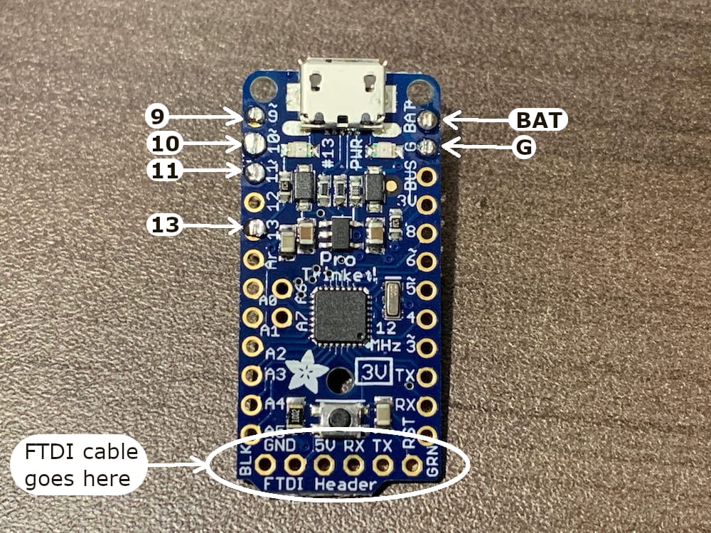
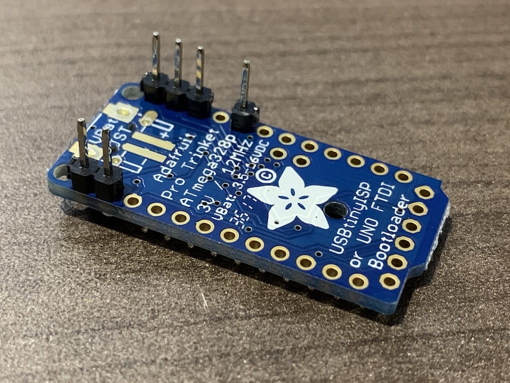
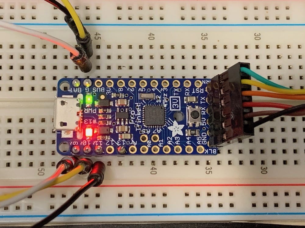
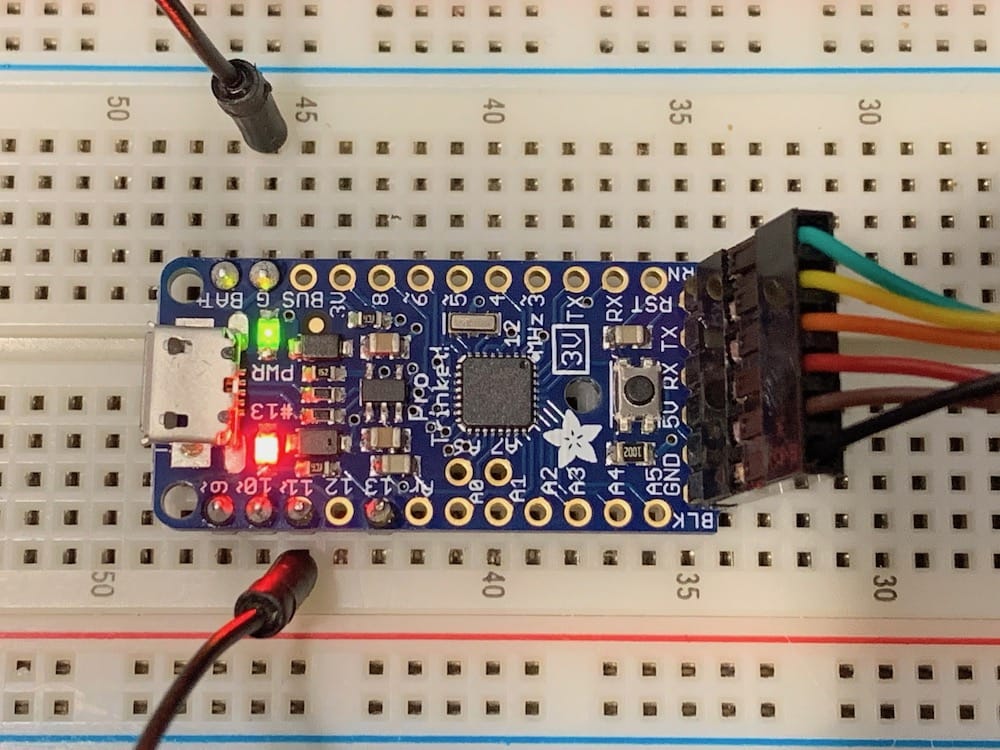
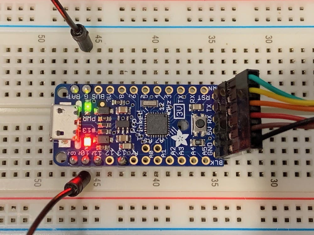
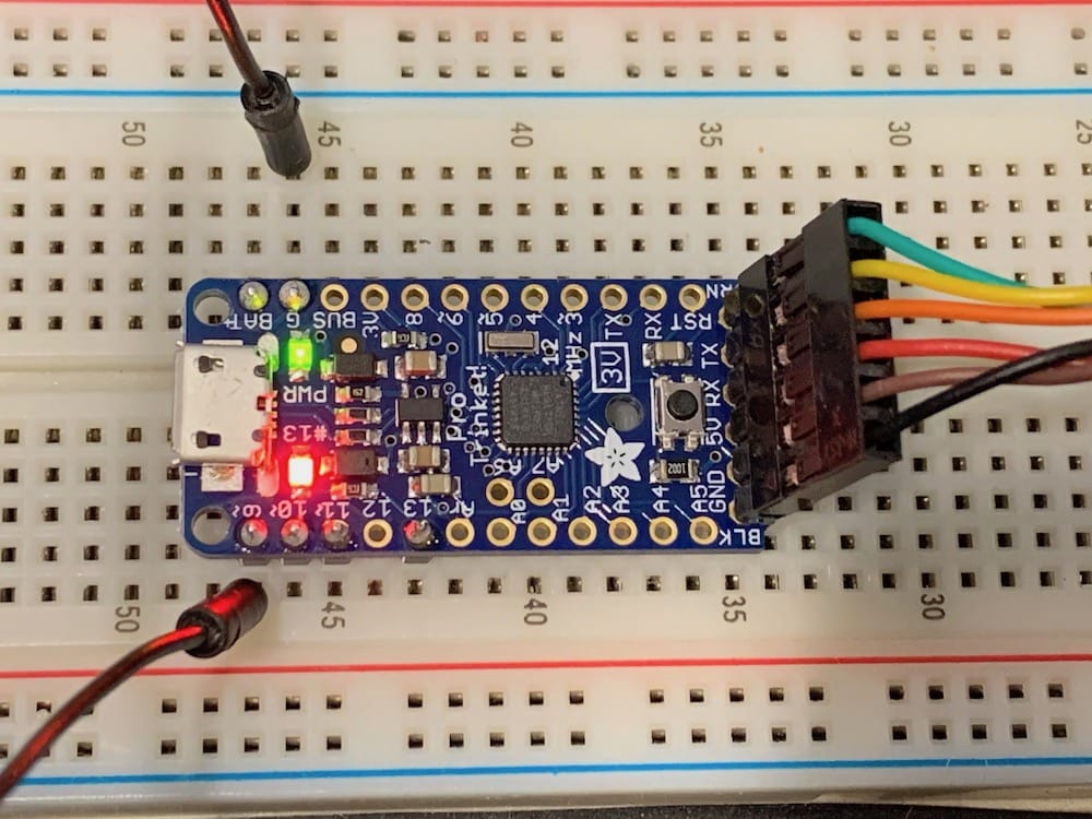
8.4. Raspberry Pi 4 Model B
A Raspberry Pi computer (RPi) is at the heart of the OpenMMS sensor. These fantastic little computers continue to evolve and have become potent devices. The functions served by the OpenMMS Raspberry Pi computer include:
Operate the simplistic LED and pushbutton User Interface
Turning on/off the lidar sensor
Starts/stops the lidar data collection and stores the raw lidar observations
Stores the real-time trajectory data from the GNSS-INS sensor
Stores the video collected by the nadir looking RPi camera (optional)
Provides a web interface for changing specific sensor parameters and for downloading the stored mission data
Many more coming soon
Refer to the OpenMMS Software section for the latest OpenMMS Operating System (OMOS) to install on the Raspberry Pi 4 Model B computer.
After the OpenMMS OS has been written to the MicroSD card, insert the card into the MicroSD slot on the bottom side of the RPi. It is strongly recommended to apply a small piece of the high-strength double-sided Nitto tape across the exposed end of the card and the MicroSD bracket. Do not remove the plastic film from the top side of the tape. Adding the tape helps ensure that the SD card renames properly seated when the OpenMMS sensor experiences any vibrations or jolts during operations and transportation. Lastly, it is also recommended to VERY CAREFULLY trim the long through-hole wires on the bottom side of the RPi beneath the two USB hubs and the ethernet jack. Trimming the excess wires helps to avoid the lidar cable from potentially being pierced by these long and sharp wires and causing issues.
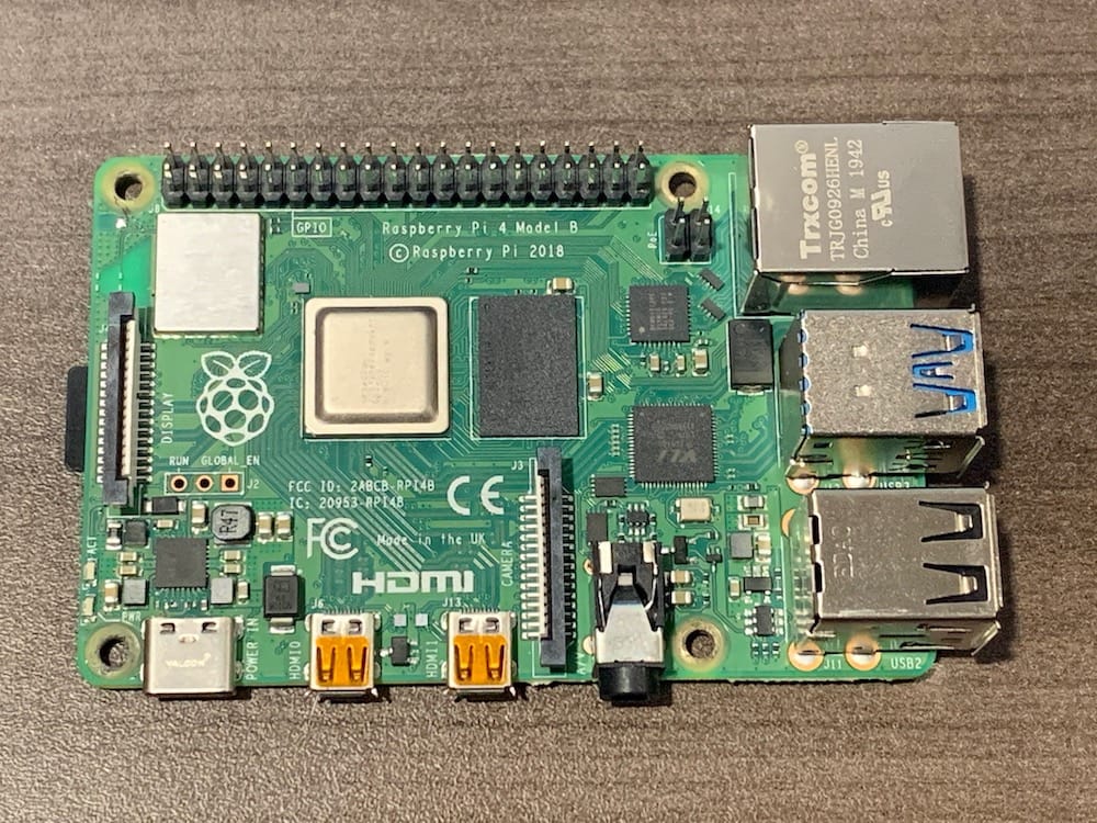
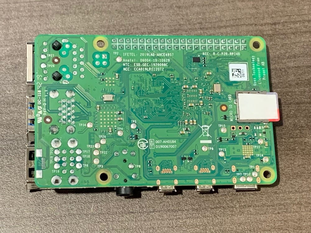
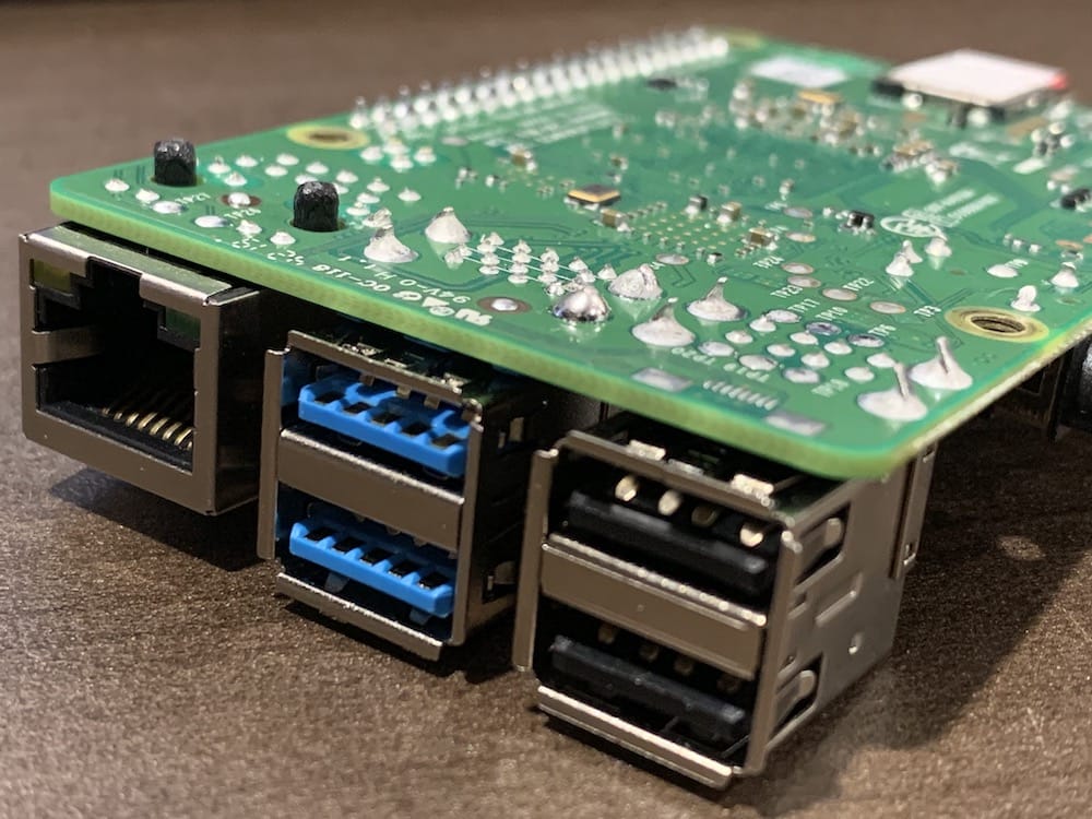
8.5. Sony A6000 Camera
The following are the recommended settings to use for the Sony A6000 Camera. The camera must be first reset to allow all readers to follow these instructions starting from the same camera state. Turn the camera on, and if prompted to set the area/date/time, follow the onscreen instructions to do so. Next, press the MENU button on the back of the camera. Refer to the images below for the steps to reset the camera.
Warning
The following Sony A6000 Camera settings are based on a Sony 16mm F2.8 pancake lens installed in the camera. If a different lens is used, it is the reader’s responsibility to ensure the appropriate camera/lens settings are applied.
There are six tabs at the top of the Menu dialog, each with a unique symbol. These instructions refer to these tabs as A, B, C, D, E, F, respectively (see Figure 8.5-1). Within each tab (except tab D), multiple pages are labeled 1, 2, 3, and so on (see Figure 8.5-2). Lastly, within each page, there are several individual setting values. The following table only lists the settings that need to be changed from their default values. The last line of the table specifies the Format function’s location, which is regularly required to delete the ‘old’ photos from the SD storage card before beginning a new mobile mapping mission.
Table H18: Sony A6000 Camera Settings
TAB
PAGE
SETTING
NEW VALUE
A
A
A
B
B
F
F
2
2
5
1
3
1
2
Flash Mode
Focus Mode
Smile/Face Detect.
Auto Review
FINDER/MONITOR
Monitor Brightness
Pwr Save Start Time
Flash Off
Manual Focus (set to inf.)
Off
Off
Monitor
Sunny Weather
30 min
TAB
PAGE
FUNCTION
DESCRIPTION
F
5
Format
Reformat SD storage card
Lastly, it is recommended that the Sony A6000 camera be set to utilize the Intelligent Auto mode. Though any photogrammetrists reading this may say otherwise! ;)
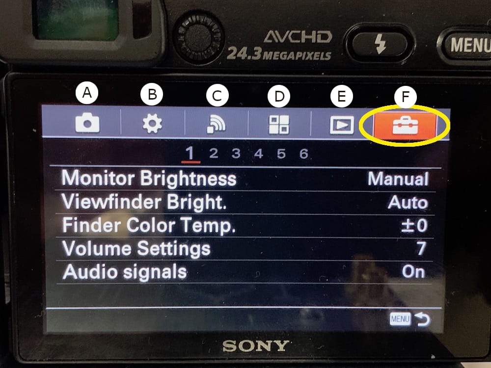
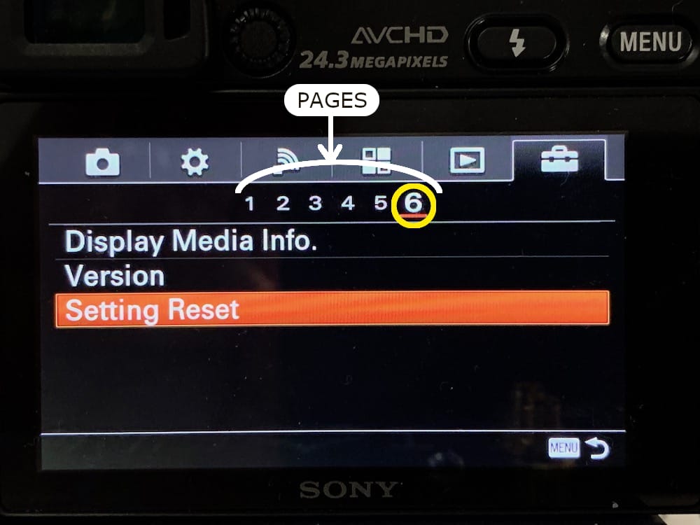
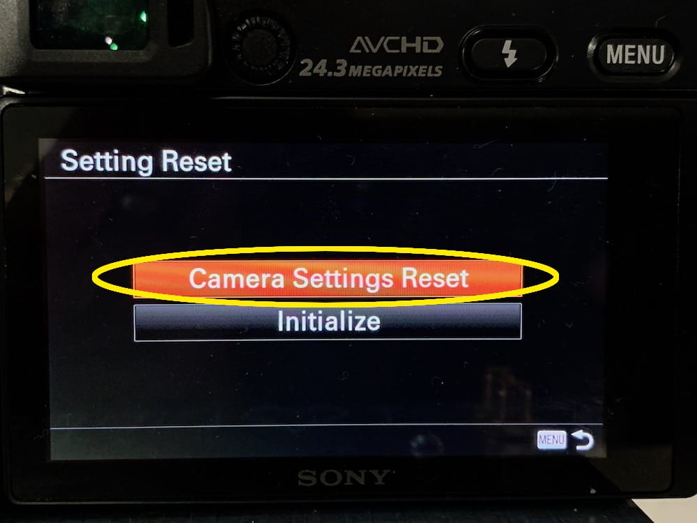
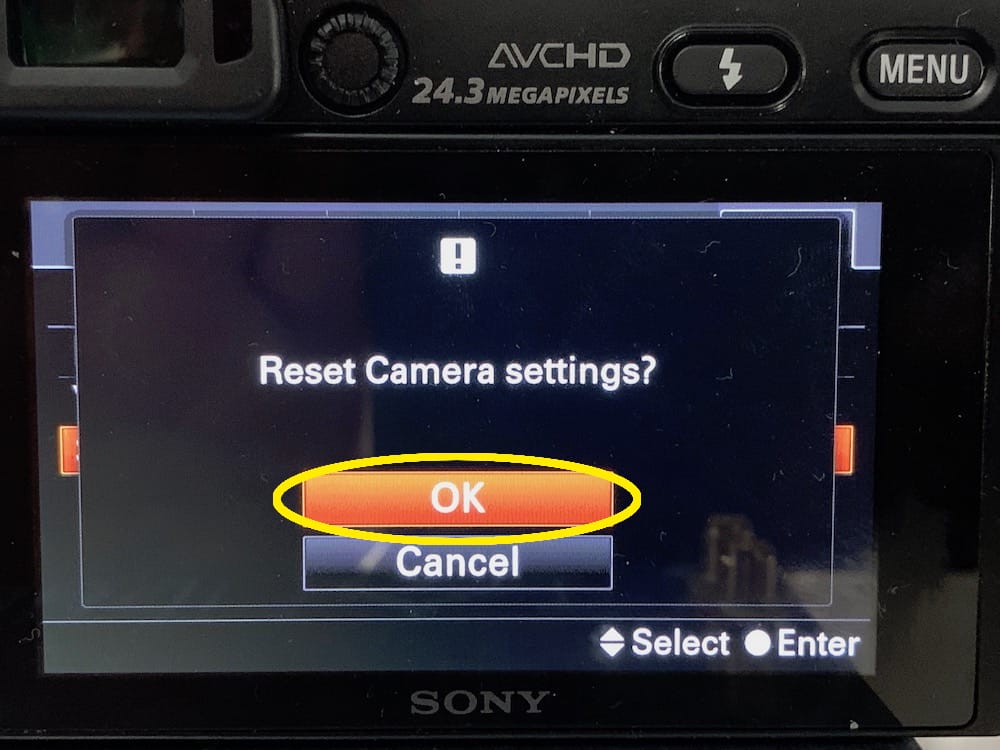
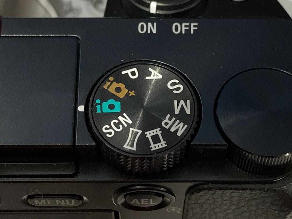

8.6. Applanix APX-18 GNSS-INS Sensor
DISCLAIMER
In this step, the expensive and sensitive Applanix APX-18 GNSS-INS sensor is used. THE READER IS RESPONSIBLE FOR ALL THE RISKS ASSOCIATED WITH THE USE OF THE APPLANIX APX-18 SENSOR!
The Applanix APX-18 GNSS-INS sensor is used to collect raw observations from GNSS satellites, along with accelerometer and gyroscope observations from the sensor’s internal Inertial Measurement Unit (IMU) while the sensor is continuously moving and rotating (i.e., kinematic motion). These observations are processed post-mission (i.e., post-processed) against carrier phase GNSS observations, from an external source, to produce position and orientation (attitude) estimates for the APX-18. This data collection and processing approach is commonly referred to as Post-Processed Kinematic (PPK). The APX-18 also provides the high precision time reference used by other OpenMMS sensor components to timestamp specific events and observations (e.g., a lidar observation). The high precision position and attitude estimates of the APX-18 sensor, at the exact moment an observation to a feature of interest was recorded by a lidar or camera sensor, allows the position of the observed feature to be directly determined (i.e., directly georeferenced).
To begin, install the two MMCX Female to SMA coaxial GNSS antenna cables onto the APX-18 sensor. Then carefully thread the two Trimble AV14 GNSS antennas onto the other end of the cables, careful not to over-tighten them. Next, install the APX-18 sensor into the 44-pin header on the Applanix development board, ensuring the mounting holes in the APX-18 properly align with the standoffs on the development board. Connect an ethernet cable to the development board and the other end directly into a computer. On the packaging for the APX-18 sensor the static IP address for the sensor should be labeled; make a note of this preconfigured IP address. Lastly, connect the power supply to the development board and then slide the POWER switch to the ON position.
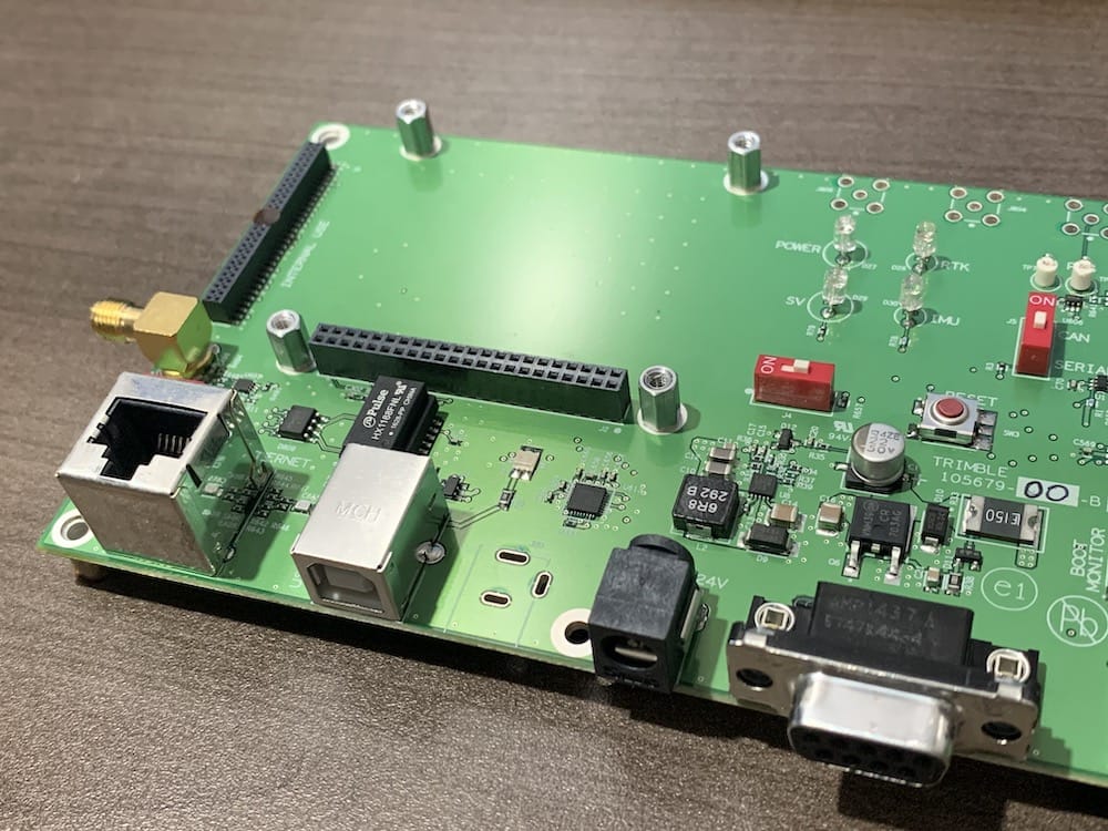
Fig 8.6-1. Development board
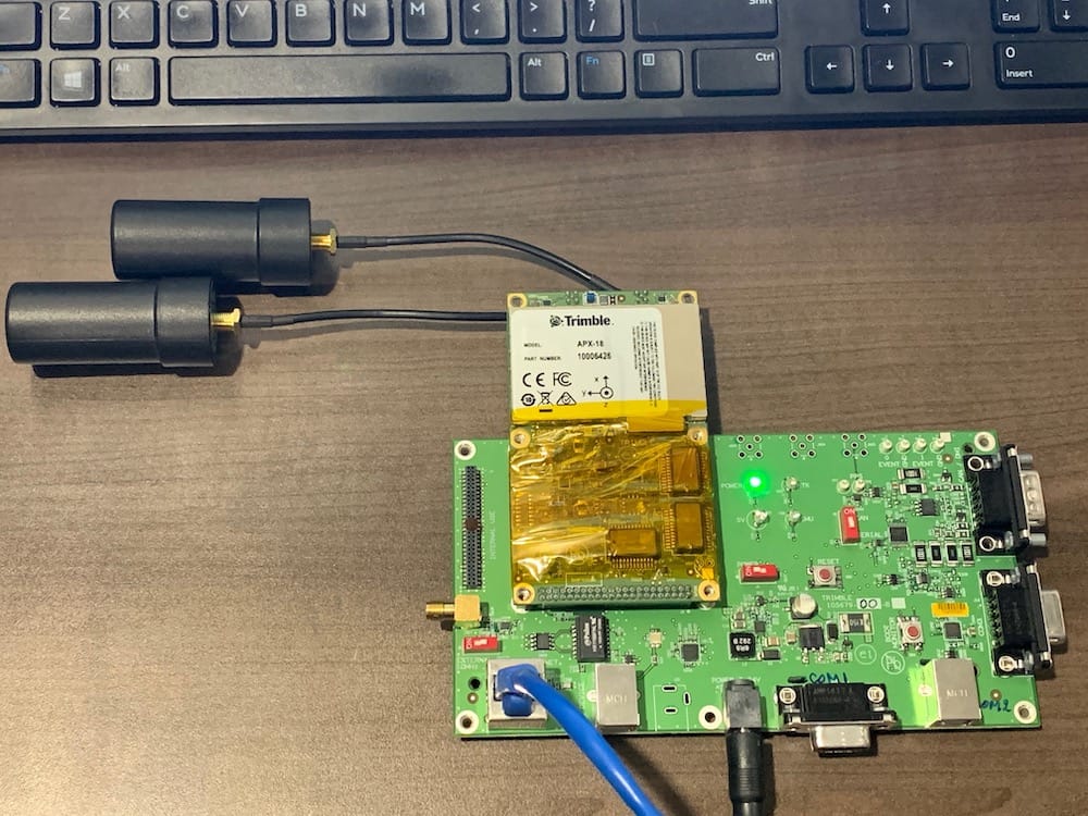
Fig 8.6-2. APX-18 installed on dev. board
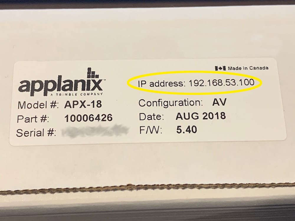
Fig 8.6-3. Preconfigured IP address
Next, the IP address of the computer being used needs to be manually configured to allow the computer to be able to communicate with the APX-18 sensor. The figure below illustrates how to set the IP address of an Apple computer manually. Windows or Linux users will have to research how to configure an IP address manually. Only the IP address and Subnet Mask need to be set. Next, open a web browser on the computer and in the URL input area type the preconfigured IP address for the APX-18 sensor. The web browser should now be displaying the APX-18 web interface. Login to the web interface using the user credentials shown in the figure below.
Attention
All the APX-18 web interface figures shown below are based on firmware version 5.5 being installed on the sensor. If a different firmware is being used, the figures below may look different. It’s the reader’s responsibility to ensure the necessary settings are still correctly configured.
There is a vast number of APX-18 configuration settings available to the end-user. However, for the current version of the OpenMMS sensor only a handful of settings need to be configured. A complete written set of instructions for configuring the new static IP address for the APX-18 will be given next. However, the remaining settings that need to be configured will only be illustrated via the figures below. PAY VERY CLOSE ATTENTION TO THE SETTINGS AND THEIR RESPECTIVE VALUES.
Begin by clicking on the Network Configuration text in the vertical column on the left side of the interface. Next, click on the Ethernet text. The ‘Ethernet Configuration’ dialog should now be displayed within the main portion of the web interface. Under the ‘Stored settings’ area, make sure that:
IP Setup setting is: Static IP
IP Address setting is: 192.168.1.200
Netmask setting is: 255.255.255.0
Gateway setting is: 192.168.1.1
Hostname setting is: OpenMMS-APX18
Remaining settings can be left to their default values
Next, click the ‘Change Configuration’ button. Lastly, on the dialog that follows, click the ‘Receiver Reset’ button to apply the new settings on the APX-18. Even though the next dialog that appears states that the APX-18 will be automatically reconnected after 60 seconds, it will not! The web browser will not automatically reconnect because the IP address has changed. Before reconnecting to the APX-18 web interface, using the new 192.168.1.200 IP address, the IP address of the computer needs to be reset to a new value to allow proper communications with the APX-18 to continue.
Tip
As the 192.168.1.0 to 192.168.1.255 range of IP addresses is very commonly used by local area networks (LANs), it is recommended that ALL other WiFi and Ethernet networks that the computer is connected to (if any) be temporarily turned Off/Disabled. By disabling other networks, any potential IP address conflicts will be avoided.
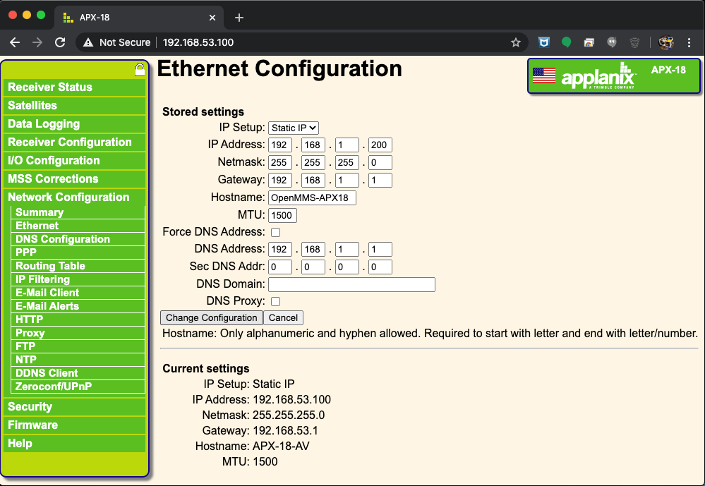
Fig 8.6-6. APX-18 ethernet settings
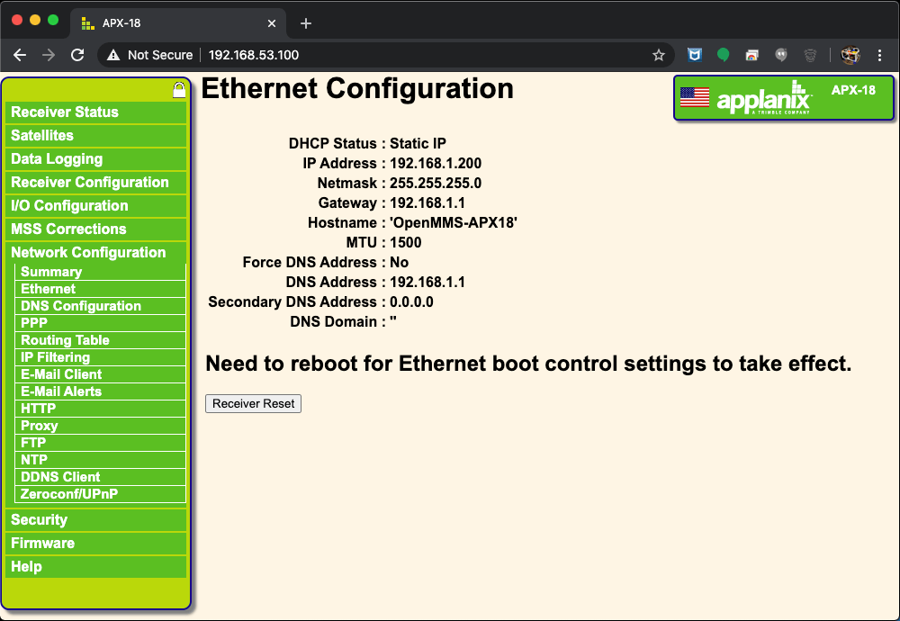
Fig 8.6-7. Reboot needed to apply new settings
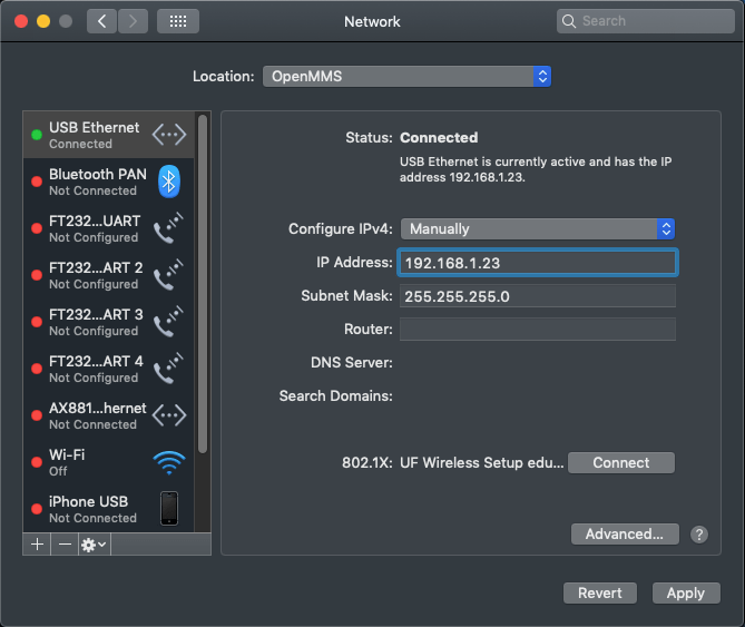
Fig 8.6-8. Reset computer IP address
Miscellaneous APX-18 Settings
After entering the respective setting value(s) on a page within the web interface, click the OK button on the page, or the settings will NOT be applied. It is strongly recommended to go back through all the pages and double-check that the settings were applied correctly.
Important
The APX-18 will be configured to automatically begin logging GNSS and inertial observations once it is powered on. Data collection is stopped by simply turning the sensor off. The sensor’s built-in 8 GB of data storage provides adequate space for most single (or even daily) mobile mapping projects. However, the APX-18 will be configured to automatically overwrite the oldest data when the sensor’s data storage becomes full.
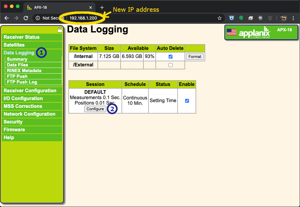
Fig 8.6-9. Data logging menu
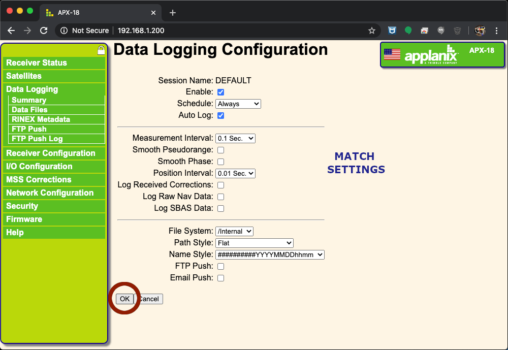
Fig 8.6-10. Data logging config.
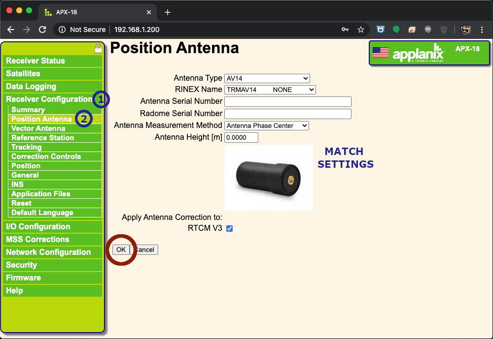
Fig 8.6-11. Position (Primary) antenna config.
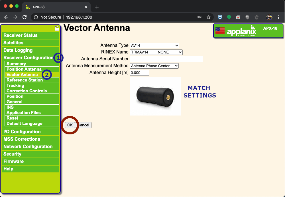
Fig 8.6-12. Vector (Secondary) antenna config.
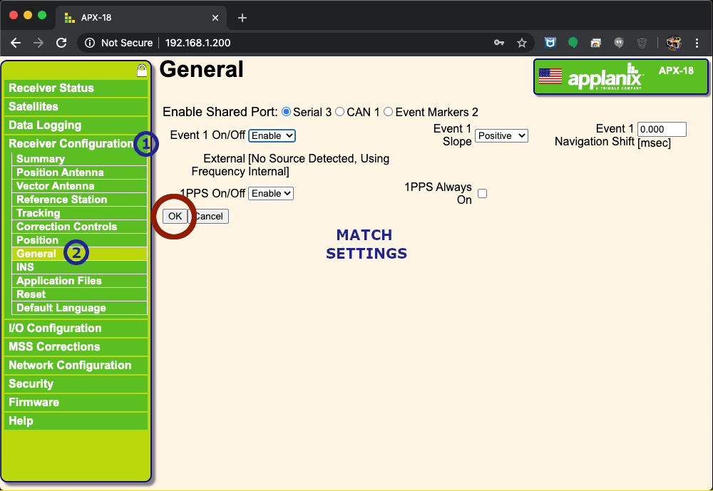
Fig 8.6-13. Event(s) and PPS config.
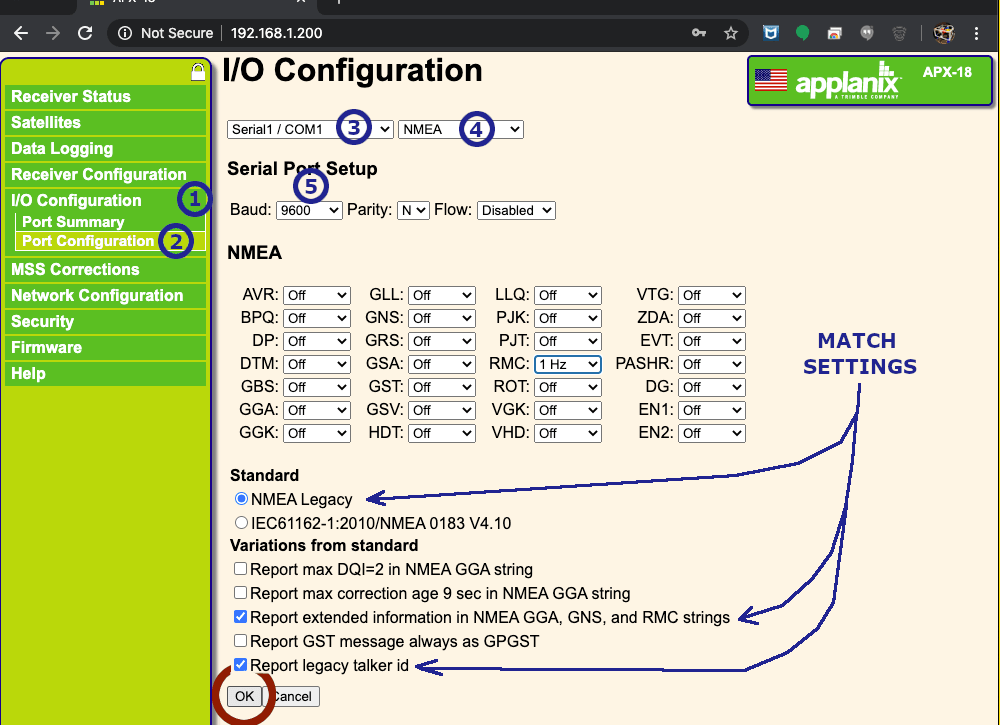
Fig 8.6-14. Serial 1 (RS232) output config.
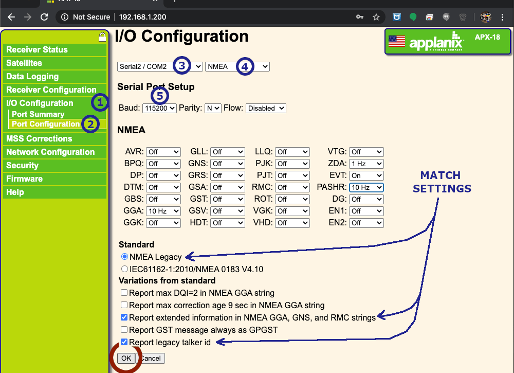
Fig 8.6-15. Serial 2 (TTL) output config.
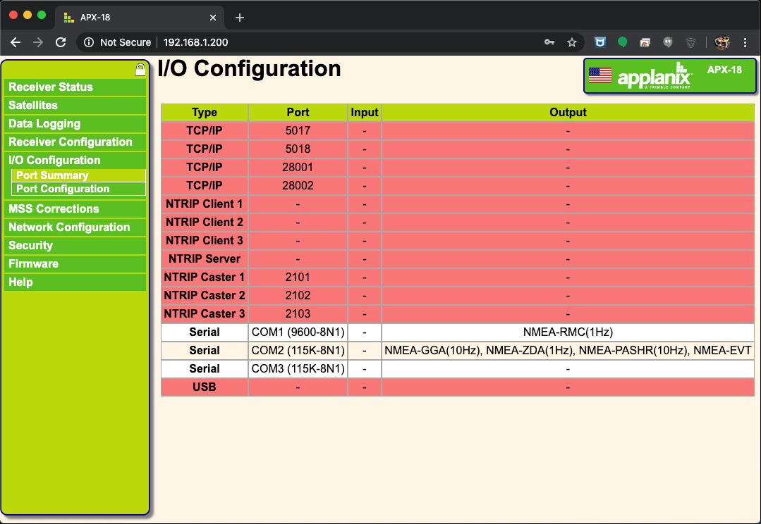
Fig 8.6-16. Verify serial output settings
APX-18 Inertial Navigation System (INS) Settings
This section of settings is critical. It is used to define the relationships between all the different coordinate frames for the individual sensors that make up the OpenMMS hardware sensor. For a reader who is new to the terms lever-arm, mounting angle, vehicle frame, etc., for the time being, it’s enough to understand that these settings allow the geospatial observations from the individual sensors to be combined to create a georeferenced point cloud.
Unlike the previous setting pages, the INS page has multiple expandable sections all on one page. The settings in all four sections should be entered before clicking the OK button at the bottom of the page. After the OK button is clicked, the web interface will prompt the user to reboot the APX-18 to apply the INS setting changes.
Attention
Some of the following INS configuration settings will probably be slightly altered after initial testing data collected with the OpenMMS sensor is post-processed and analyzed. However, due to the precise design and manufacturing of the OpenMMS sensor, the values listed below should be reasonably accurate. Calibrating the sensor involves three separate tasks (all presented in upcoming sections) and is what takes a mobile mapping system from reasonably accurate, to magical!
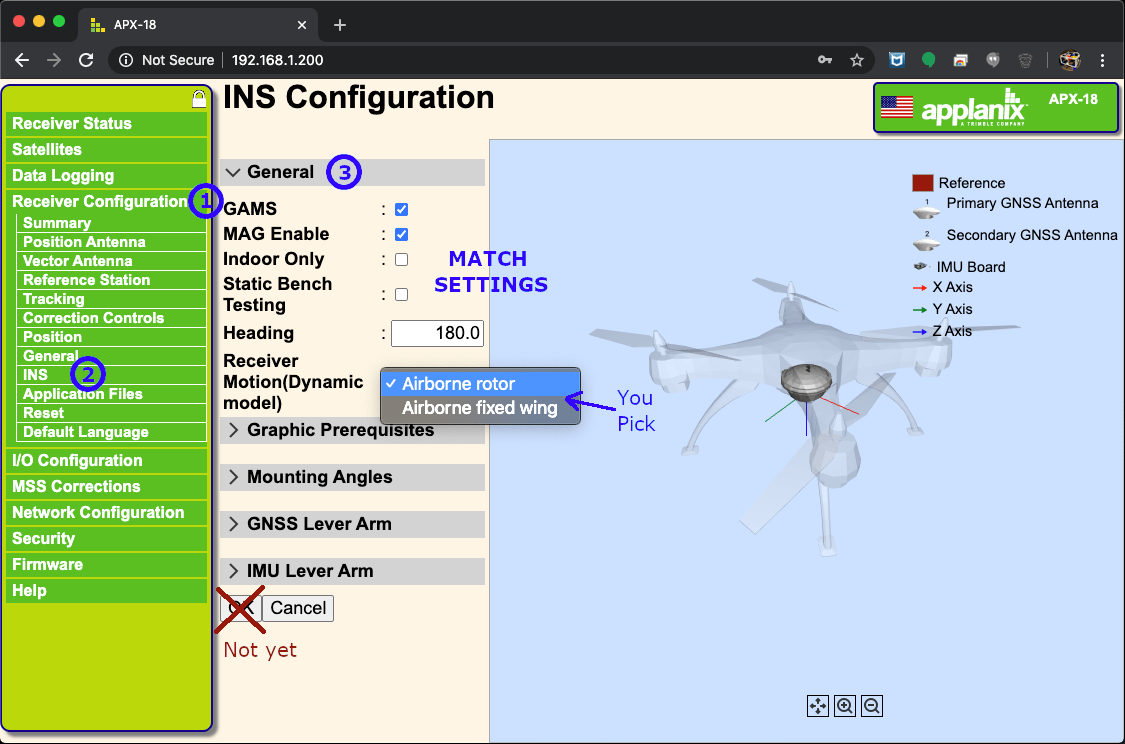
Fig 8.6-17. INS Config. - General Settings
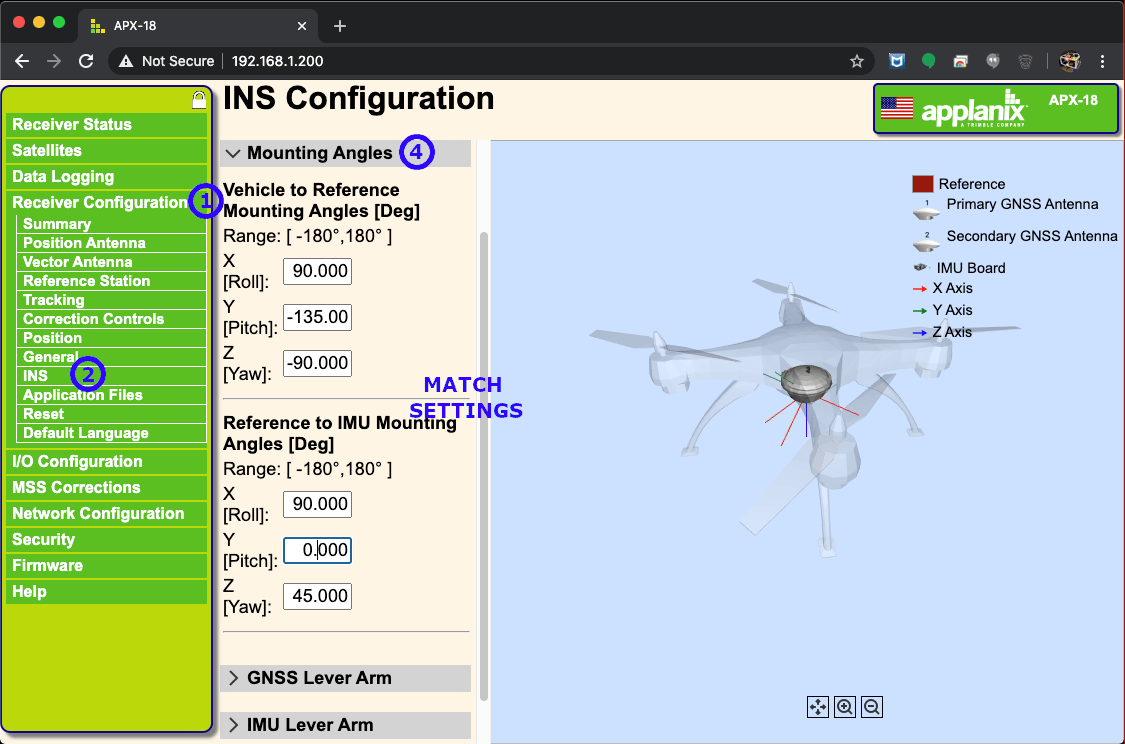
Fig 8.6-18a. INS Config. - Mounting Angles (VLP-16)
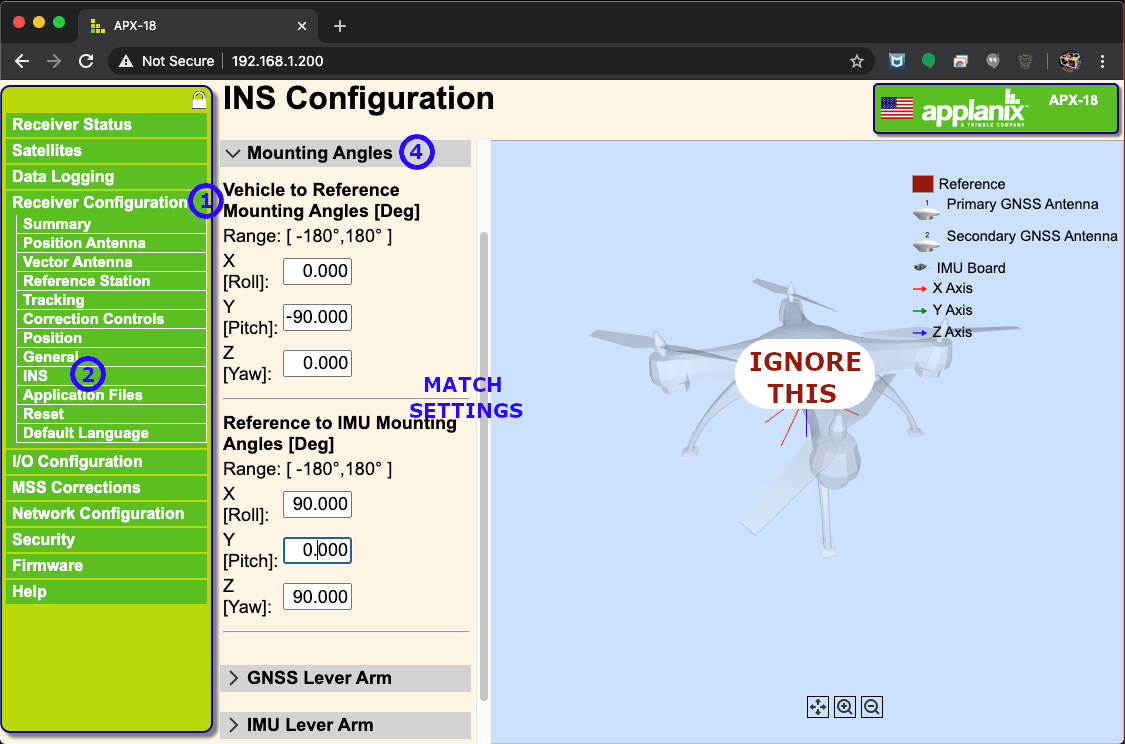
Fig 8.6-18b. INS Config. - Mounting Angles (MID-40)
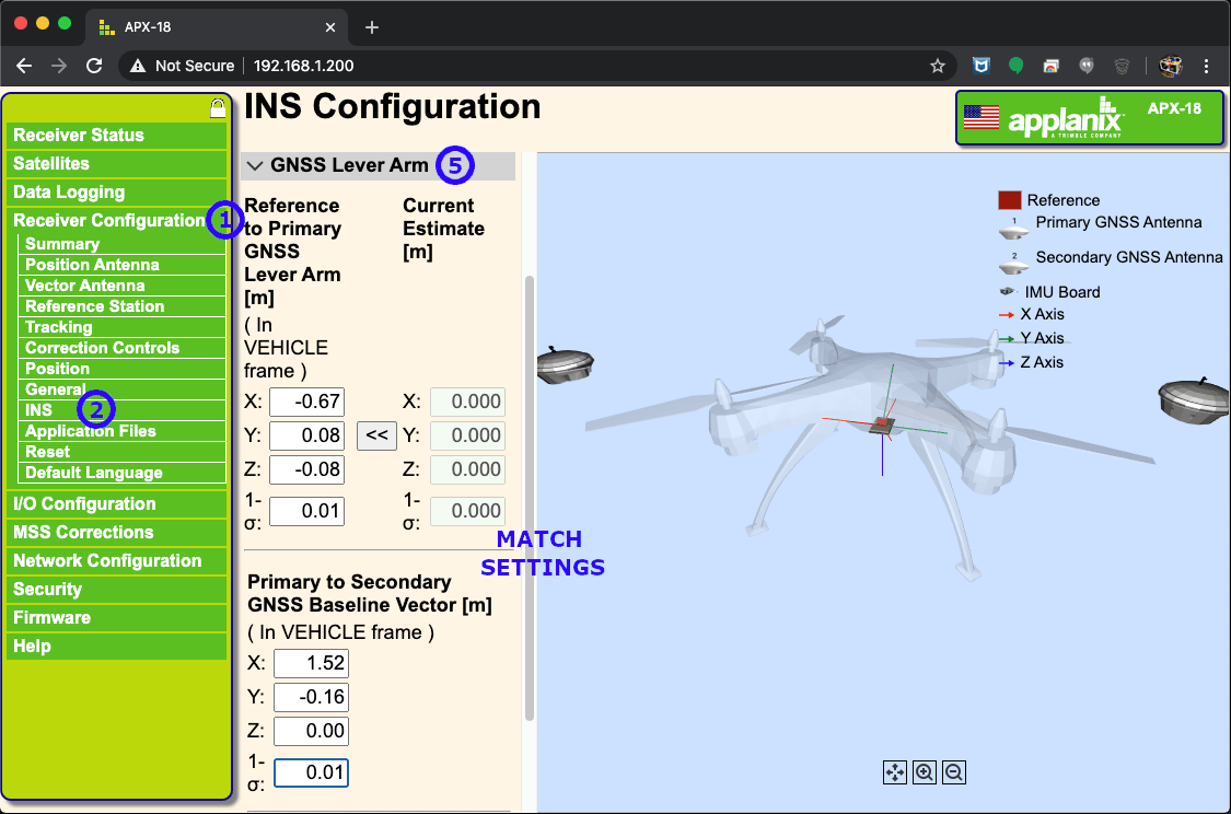
Fig 8.6-19a. INS Config. - GNSS Lever Arm (VLP-16)
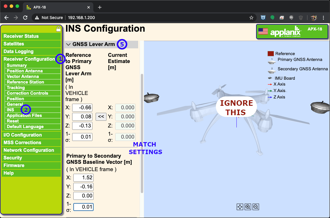
Fig 8.6-19b. INS Config. - GNSS Lever Arm (MID-40)
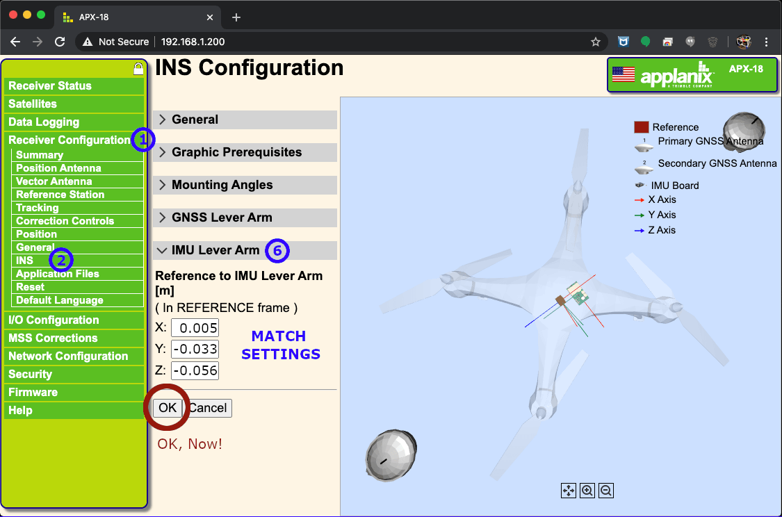
Fig 8.6-20a. INS Config. - IMU Lever Arm (VLP-16)
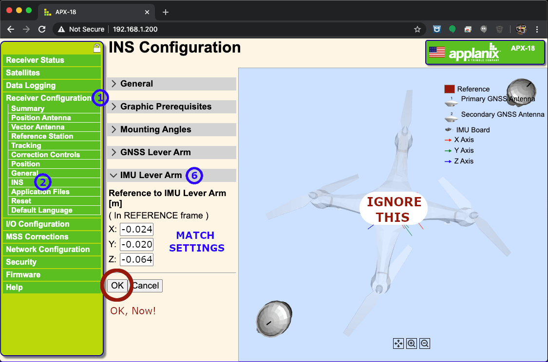
Fig 8.6-20b. INS Config. - IMU Lever Arm (MID-40)
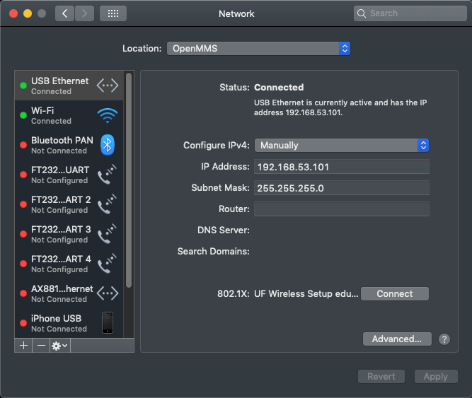
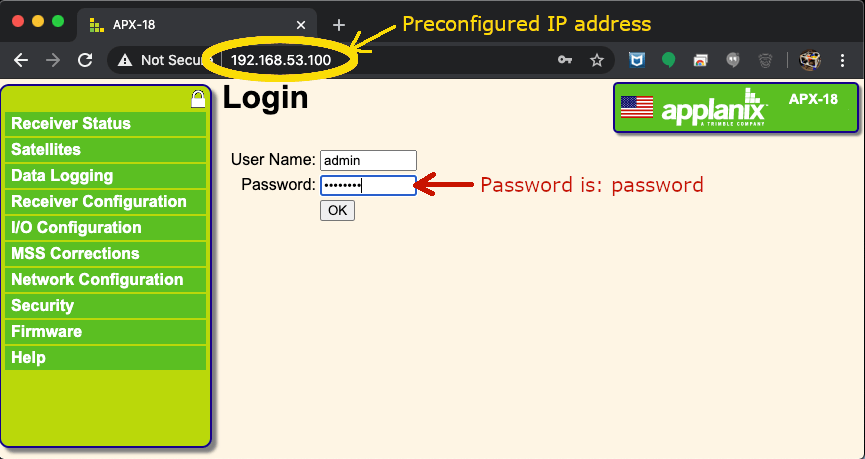
8.7. Velodyne VLP-16 Lidar
Attention
The VLP-16 web interface figure shown below is based on firmware version 3.0.40.0 being installed on the sensor. If a different firmware is being used, the figure below may look different. It is the reader’s responsibility to ensure the necessary settings are still correctly configured.
The Velodyne VLP-16 lidar sensor/laser scanner is arguably the most widely used sensor of its kind within the geospatial digital mapping domain. The VLP-16 has provided excellent reliability and measurement performance for the OpenMMS project and dozens of other commercial mobile mapping systems. Like the Applanix APX-18 GNSS-INS sensor, the VLP-16 provides a user with a web interface for configuring the sensor’s settings.
Begin by connecting the VLP-16 to the Velodyne HDL-32 Cable Adapter PCB/Interface Box (if not already connected). Connect an ethernet cable to the Interface Box and the other end of the cable directly into a computer. As discussed in the previous Applanix APX-18 Configuration section, manually set the computer’s IP address to 192.168.1.23 (or similar) and Subnet Mask to 255.255.255.0. Next, plug the power supply into the Interface Box. The VLP-16 will boot-up, and an audible hum should be heard. A mild vibration should also be felt on the sensor, which indicates the internal scanning mechanism is spinning. Next, open a web browser and in the URL input area type the preconfigured IP address for the VLP-16 sensor, which is 192.168.1.201. There are NO user credentials to enter to access the VLP-16 web interface.
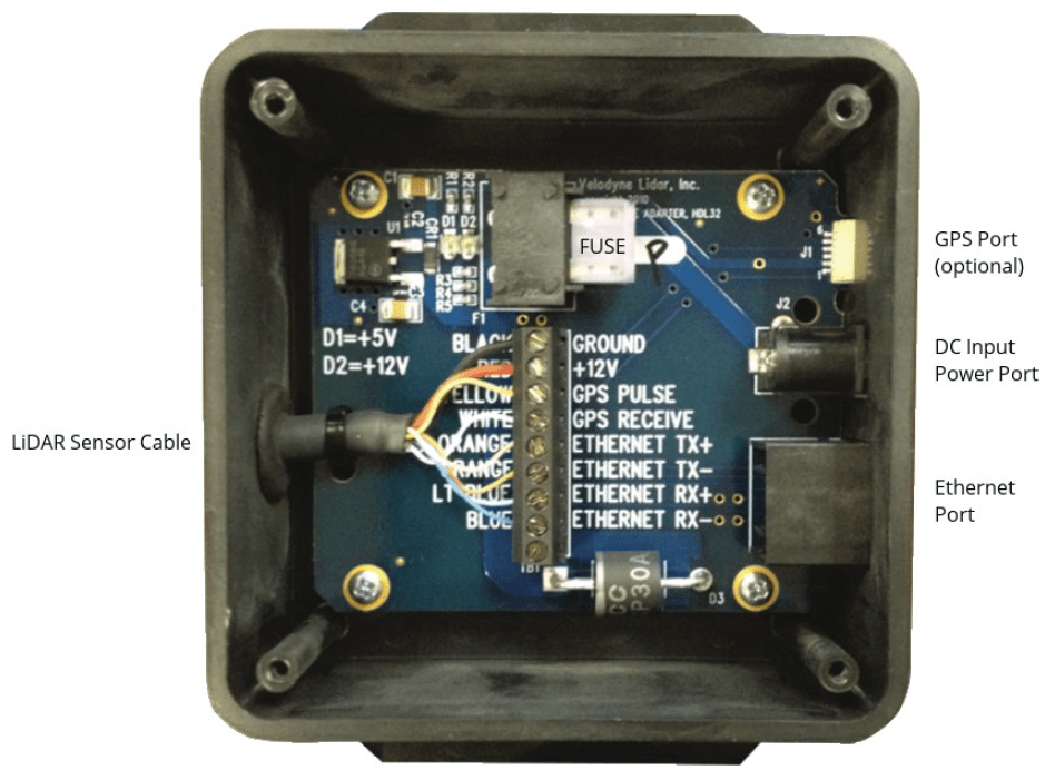
Fig 8.7-1. Velodyne Interface Box (source: Velodyne VLP-16 User Manual)
The first figure below illustrates the recommended VLP-16 settings configuration for OpenMMS sensors installed on remotely piloted aircraft systems (RPAS, a.k.a., UAS/UAV/drone). The Return Type setting MUST BE set to Dual (this is the primary benefit to using lidar). The Data Port and Telemetry Port settings MUST ALWAYS BE set to 2368 and 8308 respectively. The Motor RPM, Field of View (FOV) Start, and FOV End settings can be adjusted to meet the user’s specific needs. It is important to note that the higher the Motor RPM setting, the higher the uncertainty in the azimuth observation of each point. Because the VLP-16 is mounted at a 45-degree angle on the front face of the OpenMMS case, the FOV values require some interpretation to understand them properly. The second figure below illustrates the full range of FOV values with respect to the horizon (i.e., level surface). After the specific settings have been entered into the VLP-16 web interface, the Save Configuration button MUST be clicked. As a check, it is recommended to power down the sensor, wait until it completely stops spinning, then power it back up. Log in to the web interface and check that the desired settings are displayed.
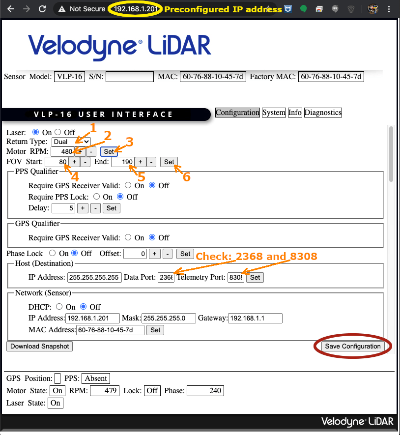
Fig 8.7-2. Velodyne web interface with recommended settings
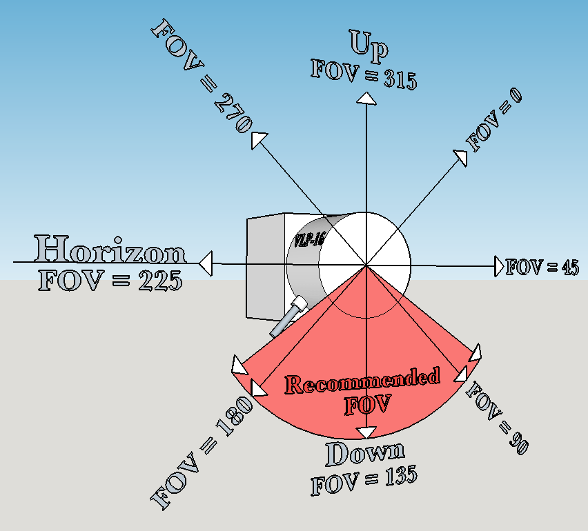
Fig 8.7-3. OpenMMS VLP-16 Field of View (FOV) values
As a final (optional) check on the VLP-16’s configuration, a user can download the free VeloView Software and install it on a computer. Open the software application and connect to the VLP-16 sensor in real-time (make sure the sensor is powered on before using the software). VeloView displays each frame (i.e., a complete scanner rotation) of data points within a 3D viewer that can be rotated, panned, and zoomed in real-time. The figure below illustrates a person sitting cross-legged in a chair, waving ‘hello’ to the VLP-16 sensor.
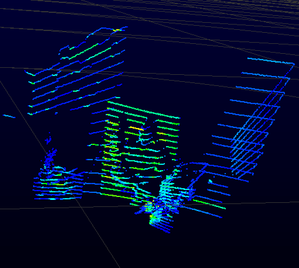
Fig 8.7-4. Screenshot of VLP-16 data viewed inside the VeloView application
8.8. Livox MID-40 Lidar
Attention
A special firmware must be installed on the MID-40 sensor in order for it to observe up to 3 returns from a single laser pulse (which is the real power of aerial lidar mapping). At the time of writing this documentation, the v03.03.0007 triple return firmware is the most recent version of the necessary special firmware. The Livox Viewer desktop application must be used to install the firmware AND configure the sensor to use a static IP address of 192.168.1.40. It is the reader’s responsibility to ensure the special firmware is installed and the IP address is configured. Refer to the Livox Viewer User Manual for details on installing firmware and setting the IP address.
To protect against the possibility of Livox removing support for this special firmware in the future, a copy of the firmware and the Livox Viewer application (for Windows OS) are included below.
The Livox MID-40 lidar sensor/laser scanner is a remarkable device! Through the tests and experiments that OpenMMS have conducted, the quality of the lidar observations made with this sensor are exceptional! Add to this, the fact that a MID-40 sensor retails for $599 USD (as of Oct. 2020) and the sensor is even more amazing, truly bleeding-edge technology!
Unlike the Applanix APX-18 GNSS-INS sensor, the MID-40 sensor does not provide a user with a web interface for configuring the sensor’s settings. In order to configure the sensor the Livox Viewer application or the Livox Software Development Kit (SDK) must be used. In an effort to simplify being able to configure and operate a Livox MID-40 lidar sensor, the OpenMMS project created an open-source Python 3 library, called OpenPyLivox (OPL), which is a near complete implementation of the Livox SDK. OpenPyLivox was designed to be a standalone library and provides the ability for anyone, from high school students interested in STEM to postdoc researchers interested in autonomous vehicles, to control a Livox lidar sensor. OPL is incorporated into the OpenMMS real-time sensor firmware and handles configuring and operating the MID-40 lidar sensor onboard the OpenMMS hardware.

Fig 8.8-1. OpenPyLivox Logo
Begin by connecting the MID-40 to the Livox Converter Box. Connect an ethernet cable to the Converter Box and the other end of the cable into a network router. A router needs to be used as MID-40 sensors are factory set to use a DHCP assigned (i.e., dynamically assigned) IP address. Ensure that the computer being used to run the Livox Viewer application is also connected to the same network router (wired or wireless). Lastly, connect a 12V power supply to the Livox Converter Box. The MID-40 will boot-up, and an audible hum should be heard. It may be possible that it sounds a bit like something is grinding inside the sensor at initial startup. The OpenMMS project contacted Livox about this sound and were assurred that the grinding sound was normal. From our test the lidar sensor appears to perform very well even when the grinding noise was present. Next, open the Livox Viewer application and, assuming all the network connections are correct, the MID-40 sensor should appear in the left column of the application. Follow the instructions provided in the Livox Viewer User Manual for details on how to install the 03.03.0007 special firmware and set the IP address to a static 192.168.1.40. The figure below illustrates a person sitting cross-legged in a chair, waving ‘hello’ to the MID-40 sensor.
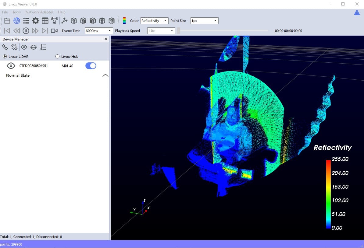
Fig 8.8-2. Screenshot of MID-40 data viewed inside the Livox Viewer application
CONGRATULATIONS!
YOU HAVE NOW FINISHED CONFIGURING ALL THE COMPONENTS!
9. Carbon Fiber Parts Assembly
Danger
Machining parts from carbon fiber material can create potentially hazardous carbon fiber dust in the air. It is the responsibility of the person(s) using these instructions to produce their own (i.e., the manufacturer of an) OpenMMS sensor, to ensure that satisfactory air quality requirements are met or exceeded, during any process discussed within these instructions when working with carbon fiber material.
9.1. Overview
In this section, the carbon fiber GNSS antenna ground planes are attached to the carbon fiber GNSS antenna arms and the GNSS antenna cables are installed within the arms.
9.2. GNSS Antenna Arms
The following components are needed to assemble the GNSS antenna arms.
2 @ 20mm x 20mm x 800mm carbon fiber square tubes
2 @ OpenMMS GNSS antenna ground planes
2 @ OpenMMS GNSS antenna cables (~100cm in length)
2 @ Trimble AV14 GNSS antennas
6 @ 3mm (M3) buttonhead bolts, 8mm in length with Nyloc nuts (not shown)
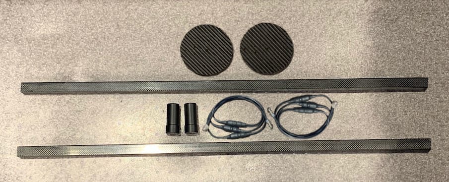
Fig 9.2-1. Components needed to assemble the GNSS antenna arms
Begin by positioning the center point at the end of the square tubing approximately 8mm from the center hole in the ground plane. Mark the locations of the three mounting holes of the ground plane on the top side of the square tubing. Use either the Proxxon Drill Press or a handheld electric drill, and drill through the topside of the square tubing at the locations of the mounting holes (do NOT drill through both the top and bottom sides of the tubing). Next, insert three M3 8mm long bolts through the ground plane and then through the tubing’s top side. Use a small set of pliers to hold a Nyloc nut inside the tubing and then tighten the respective M3 bolt. Repeat this process on the 2nd GNSS arm.
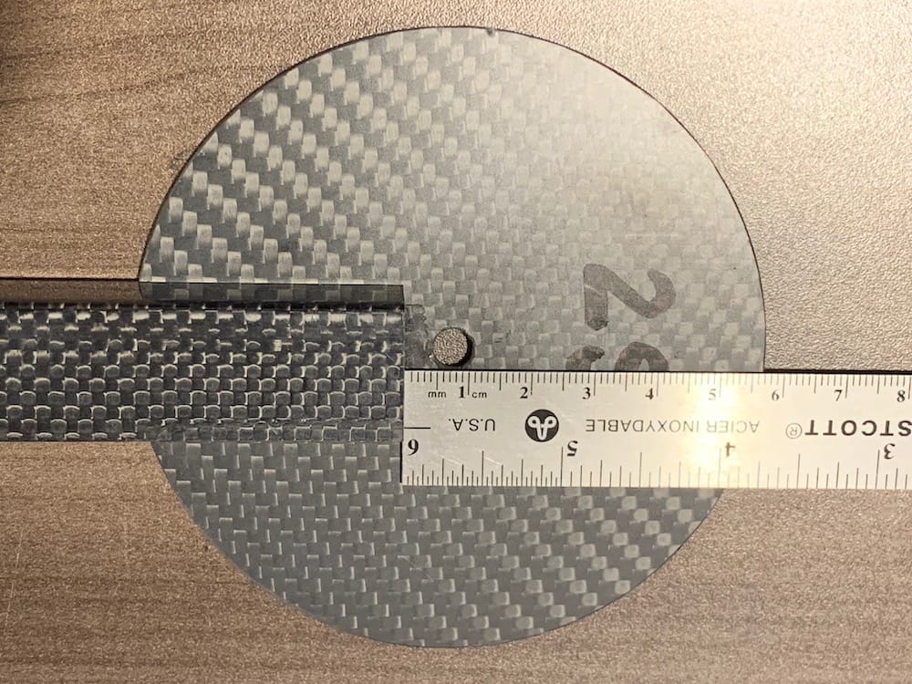
Fig 9.2-2. GNSS arm on the ground plane
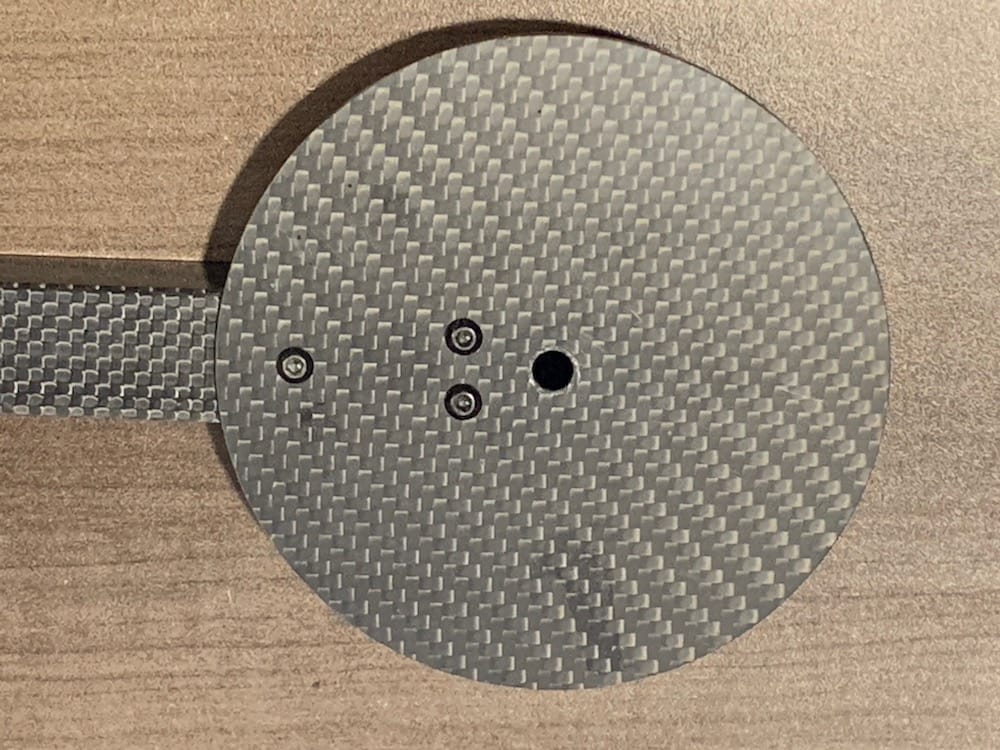
Fig 9.2-3. Holes drilled, bolts inserted
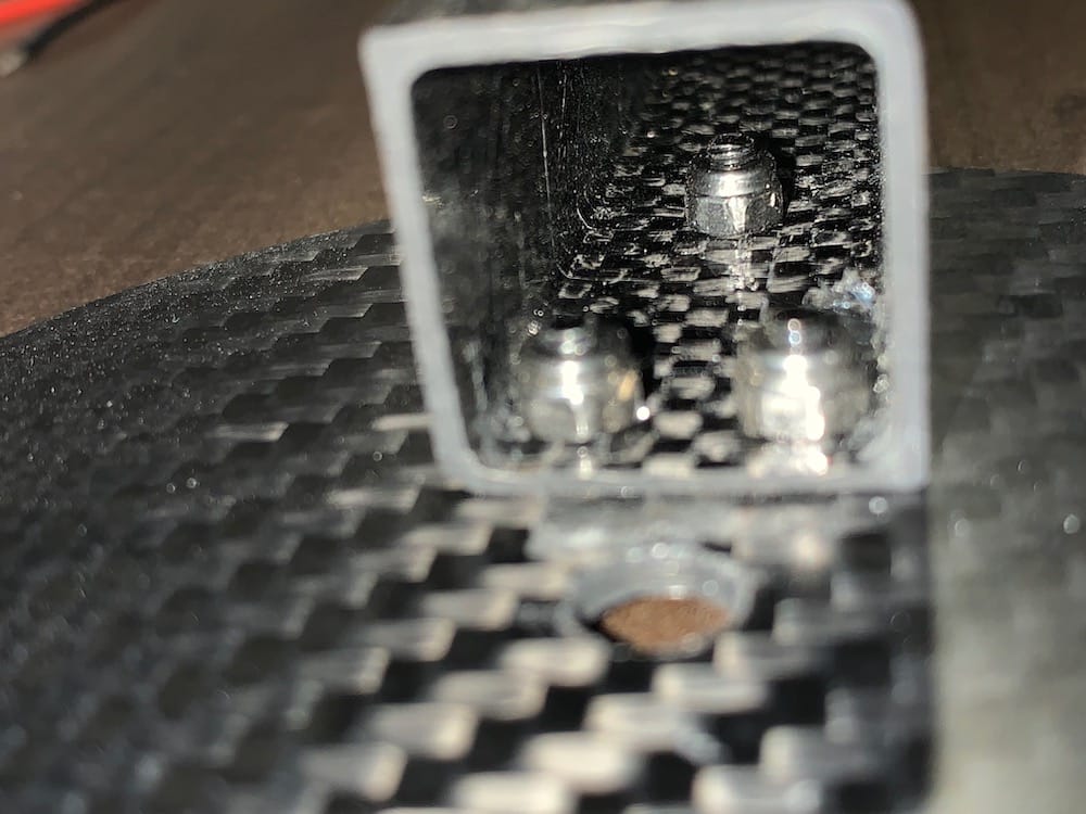
Fig 9.2-4. Nyloc nuts inside GNSS arm
Next, position one of the GNSS arms, so the ground plane is on the right side of the arm, and the ground plane is facing up. From the end of the GNSS arm without the ground plane, measure approximately 12 cm along the inside face of the square tubing (i.e., the side of the tubing facing you). Mark a line across the face of the tubing at the 12cm measurement. Using a handheld electric drill, drill a small pilot (~1/8” bit) at the midpoint of the line (do NOT drill through both sides of the tubing). Gradually widen the drilled hole until it reaches a diameter of 1/2”. Next, remove the locking nut and the star washer from the male ends of the GNSS antenna cables. Insert the male end of a GNSS cable into the drilled hole and push it until it comes out of the tubing beneath the ground plane. The other GNSS arm does NOT require a hole drilled into it. Rather the GNSS antenna cable runs the entire length of the arm. Insert the male end of the GNSS antenna cable into the end of the tubing without the ground plane and then push it until it reaches the other end beneath the ground plane. Next, insert the male end of the cable through the center hole in the bottom of the ground plane. Replace the star washer and locking nut on the end of the cable and then tighten the locking nut. Repeat this process on the other GNSS arm. It is recommended to create a small tension loop in each GNSS antenna cable directly underneath the ground plane. Use a small zip-tie to secure the loop. The tension loop helps avoid the antenna cable being damaged in the event the cable is pulled too tightly from the exposed end. Lastly, visually observe the location where each GNSS antenna cable comes out of each respective GNSS arm. Install one or more layers of heat-shrink tubing at these locations on the antenna cables. The heat-shrink tubing helps protect the cable from being damaged by repetitive movement/friction with the edges of the carbon fiber GNSS arms.
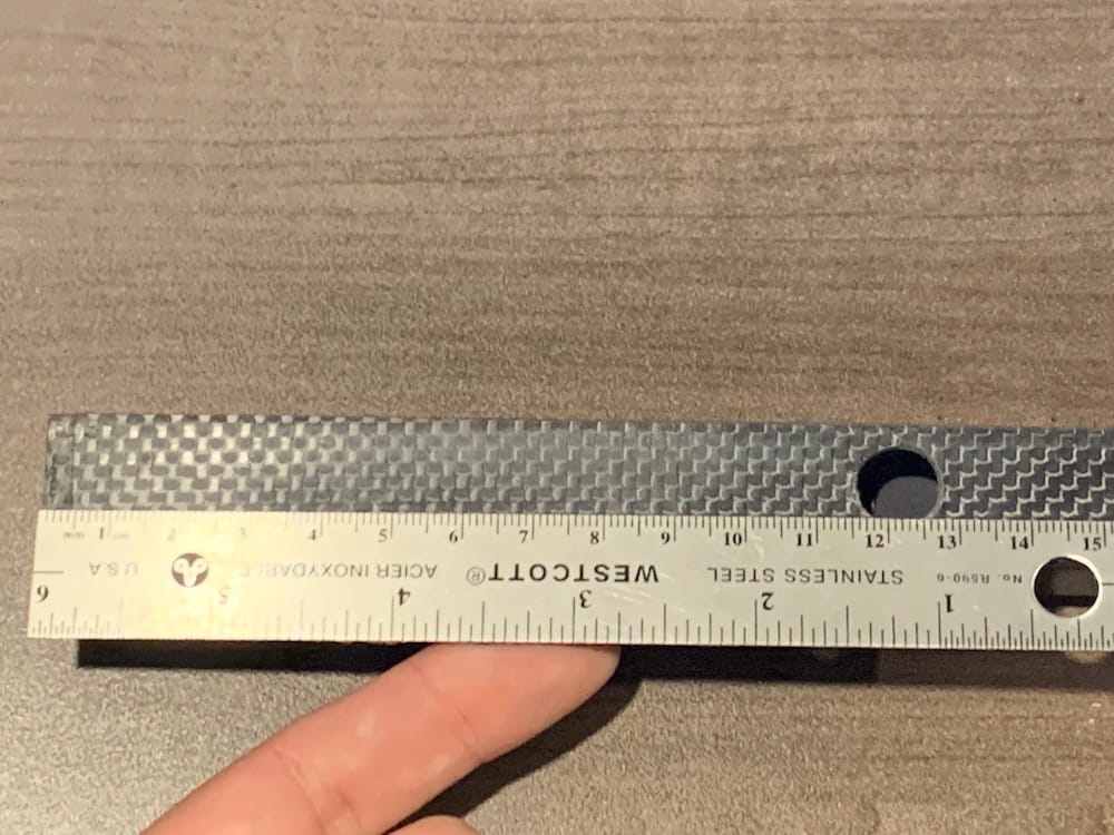
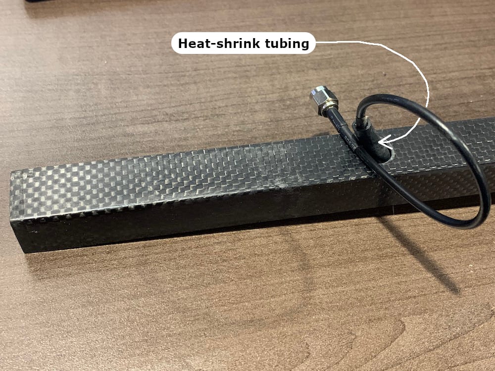
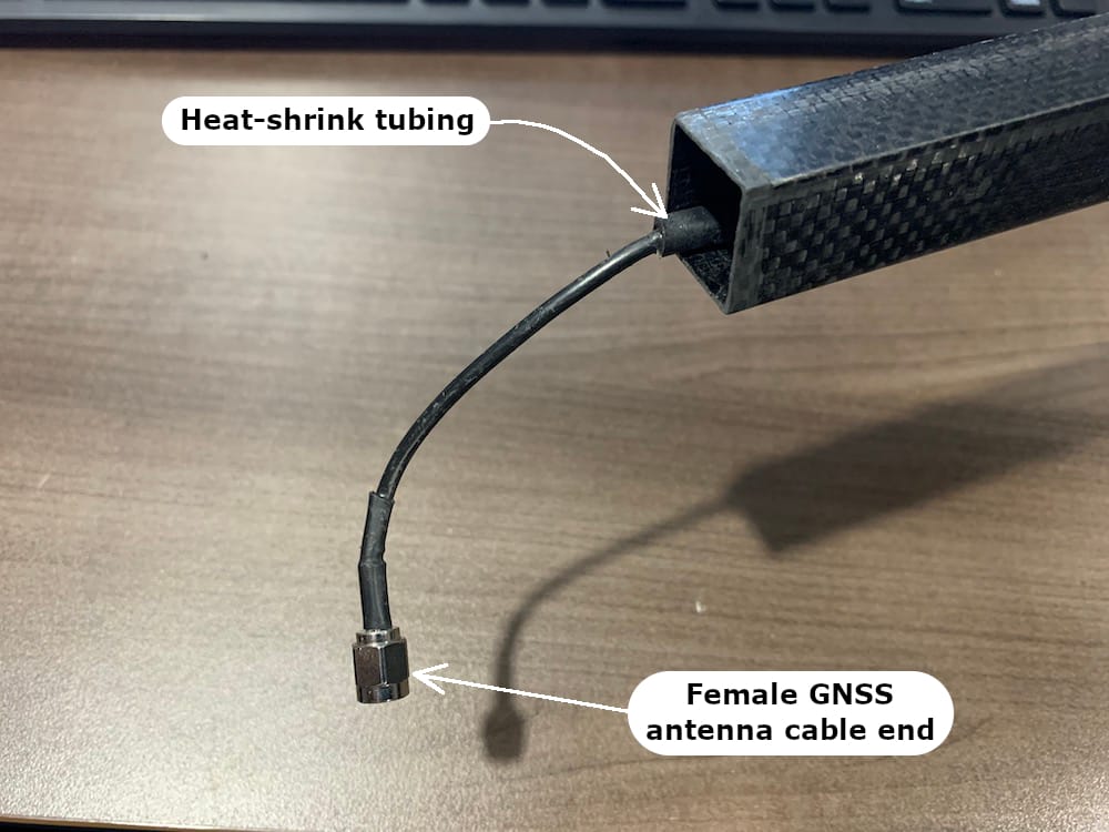
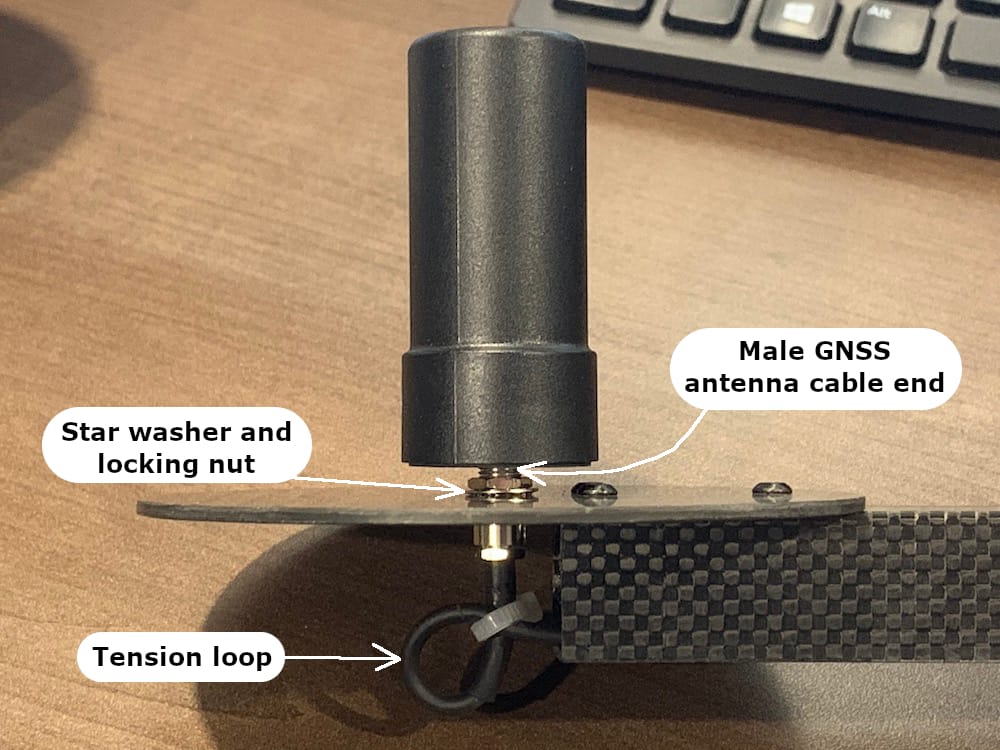
CONGRATULATIONS!
YOU HAVE NOW FINISHED ASSEMBLING ALL THE CARBON FIBER PARTS!
10. Printed Circuit Boards Assembly
10.1. Overview
In this section, the three manufactured printed circuit boards (PCBs) are populated with all of their small electronic components by hand soldering them into place. It is recommended to assemble the PCBs in the exact order of operations, as discussed below. Pay very close attention to the instructions and the details highlighted within the figures. Several components can potentially be installed on the PCBs in different ways, but ONLY one way is correct. Lastly, the Bantam Tools Machine cannot manufacture PCBs with plated through-holes (i.e., the soldering pads aligned with each other on the top and bottom layers of the PCB are NOT connected with copper). Due to this, in combination with trying to minimize the number of vias in each PCB, some components must be solder on the top layer, the bottom layer, or both layers.
Tip
Use a precision tip soldering iron.
Use a higher heat setting for the soldering iron, and this will significantly help with soldering ground plane connections.
Keep the soldering tip very clean.
Use high-quality flux core solder.
10.2. LED Board
The following components are needed to assemble the OpenMMS LED Board v1.3.
1 @ 2x5 ribbon cable jack
4 @ 5mm LEDs (recommended to be blue)
1 @ 5mm RGB LED (must be common anode)
4 @ 330 ohm through-hole resistors (1/4 Watt)
1 @ 1.5 Kohm through-hole resistor (1/4 Watt)
1 @ 3.0 Kohm through-hole resistor (1/4 Watt)
1 @ 4.7 Kohm through-hole resistor (1/4 Watt)
OpenMMS LED Board v1.3
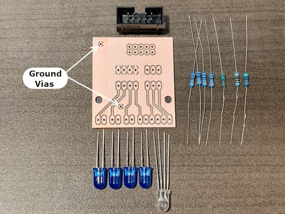
Fig 10.2-1. Components needed to assemble the LED Board
Begin by installing the seven resistors into their respective holes on the top layer of PCB. Resistors do not have polarity, so it does not matter which end goes where. Refer to the LED Board - interactive PCB viewer in section 5.4 for details on which resistor goes where. The resistors only need to be soldered to the lower pads on the top layer. Now flip the PCB over to the bottom layer. The resistors only need to be soldered to the upper pads of the bottom layer. Trim the excess wire from the legs of the resistors. Next, insert a small piece of wire (the excess resistor wire works well) through the two ground vias and solder them to the bottom layer. Flip the PCB over to the top layer and solder the wires in the ground vias to the top layer. Trim any excess wire from both sides of the PCB.
Next, insert the 5mm LEDs (1 RGB and 4 Blue) into the holes on the bottom layer of the LED Board. Pay close attention to the legs of the LEDs, as shown in the following figure. LEDs have polarity and need to be installed correctly. Next, take two 3mm (M3) button-head bolts 5mm in length, and insert them into the two holes on the OpenMMS right face that are just above the 5 LED holes (refer to figure 4.6-2). On the inside of the right face, install an M3 female/female standoff 6mm in length, onto each bolt. Position the LED Board roughly over its correct location on the inside of the right face, and then fully insert the individual LEDs into their respective holes through the aluminum. While ensuring the LEDs stay properly seated within the right face, begin pushing down on the LED Board and adjusting the individual LED legs. Continue until the LED Board’s mounting holes align with the standoffs. When possible, insert two M3 button-head bolts, 5mm in length, through the mounting holes, and fully seat the LED Board to the standoffs.
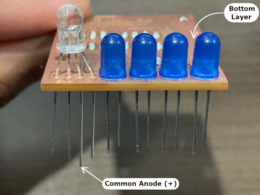
Fig 10.2-4. LEDs in bot. layer
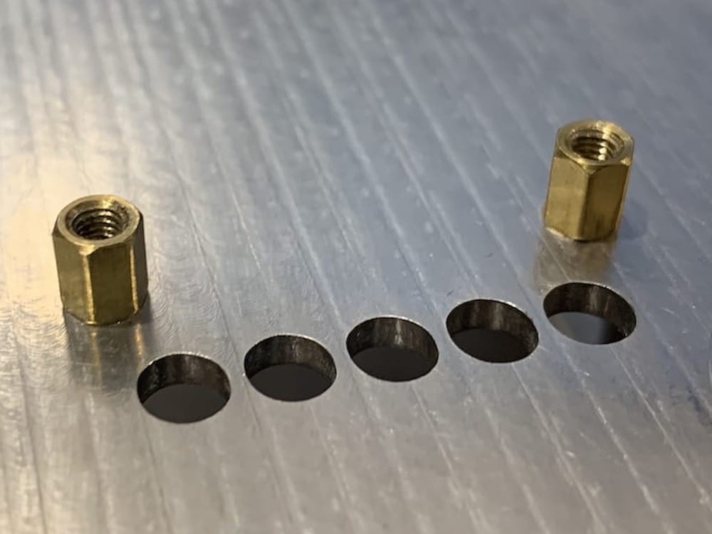
Fig 10.2-5. Standoffs installed
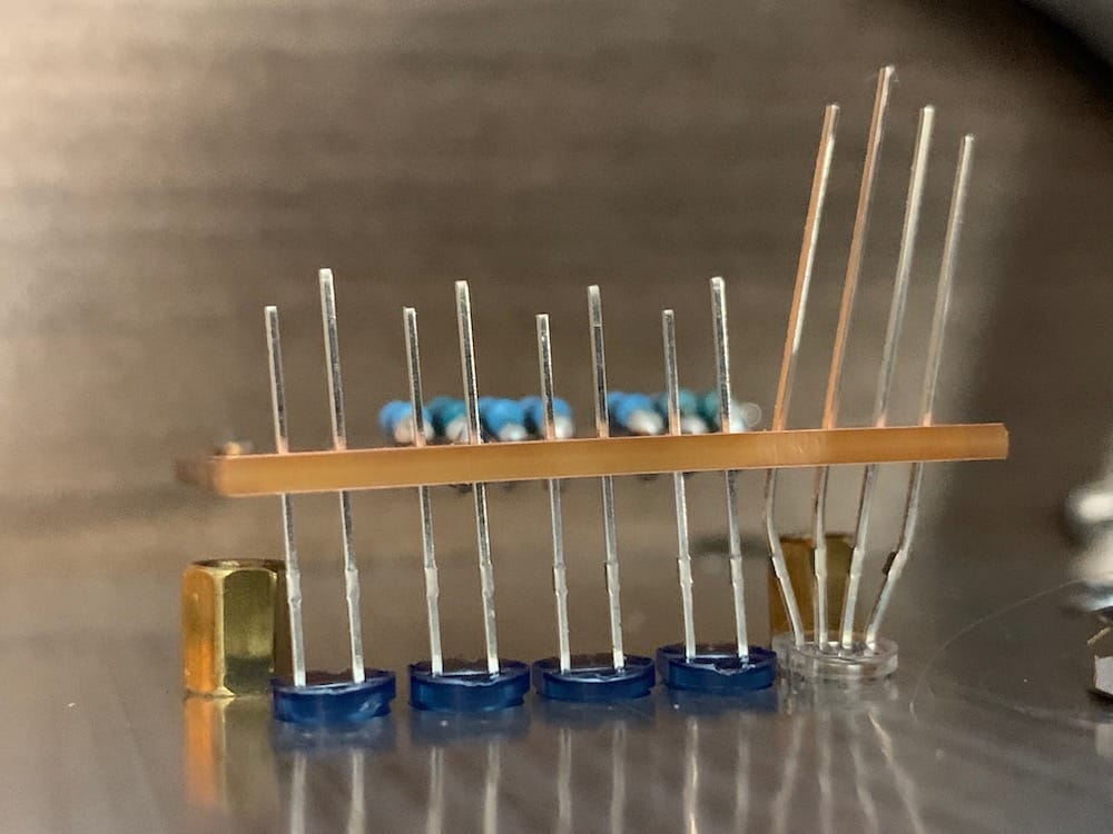
Fig 10.2-6. LEDs in the right face
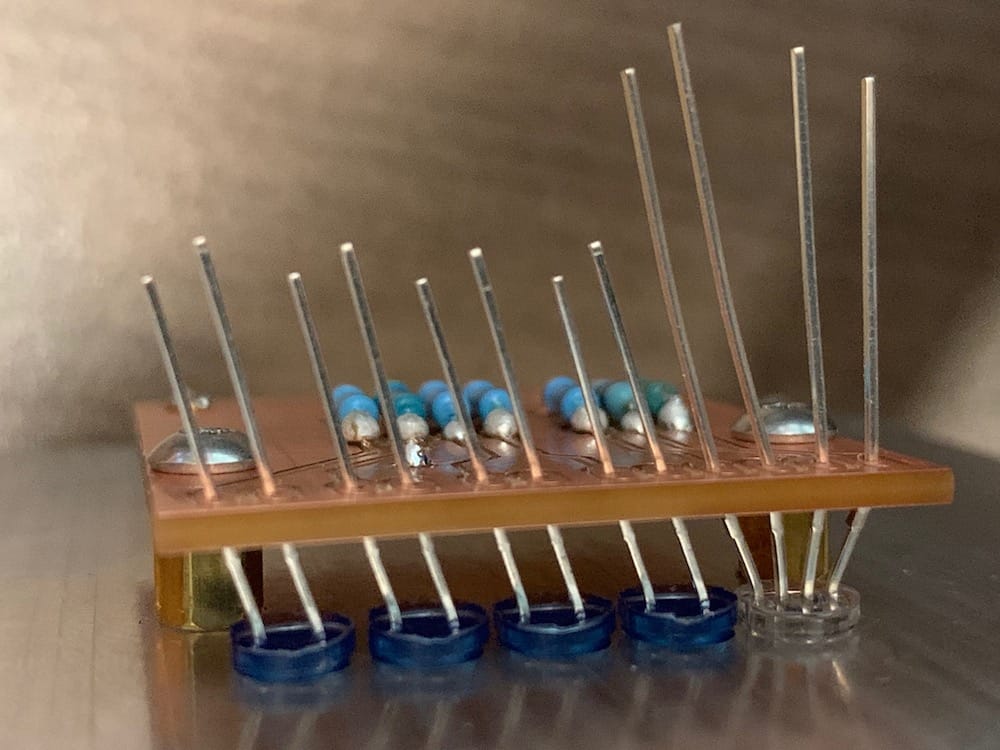
Fig 10.2-7. LED Board installed
Next, with the LED Board bolted in place, and the LEDs still properly seated, the twelve LED wires are soldered to their respective pads on the top layer. Trim the excess LED wires. Unbolt the LED Board from the right face and carefully remove it. Gently push on the LEDs sticking out of the right face to easily remove the LED board. Next, on the bottom layer of the LED Board, the anode (positive voltage) wires for each of the five LEDs needs to be soldered to its bottom layer pad (see the figure below). These solder connections can be a bit difficult to make. Take your time, avoid damaging the LED with the soldering iron, and avoid creating any short circuits. Finally, install the 2x5 ribbon cable jack into the top layer of the board and be sure that the jack’s reference mark is towards the upper edge of the LED Board. Solder the ten pins of the jack to the bottom layer.
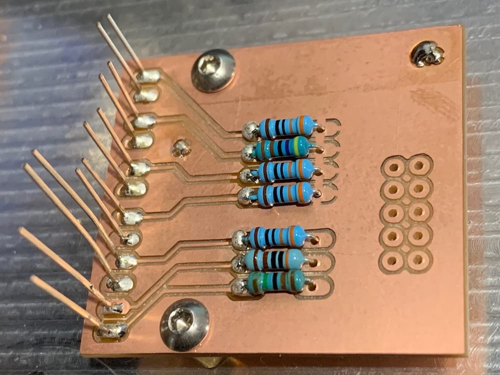
Fig 10.2-8. LEDs soldered to the top layer
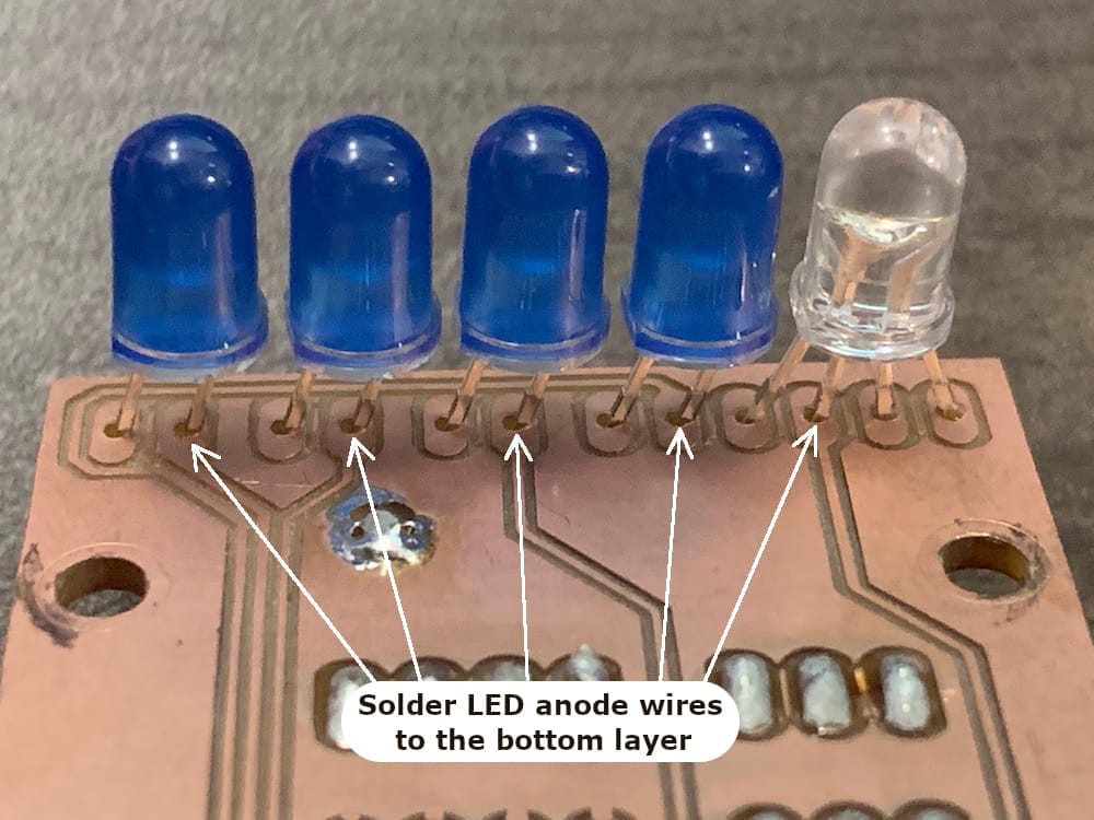
Fig 10.2-9. LED anode wires to solder
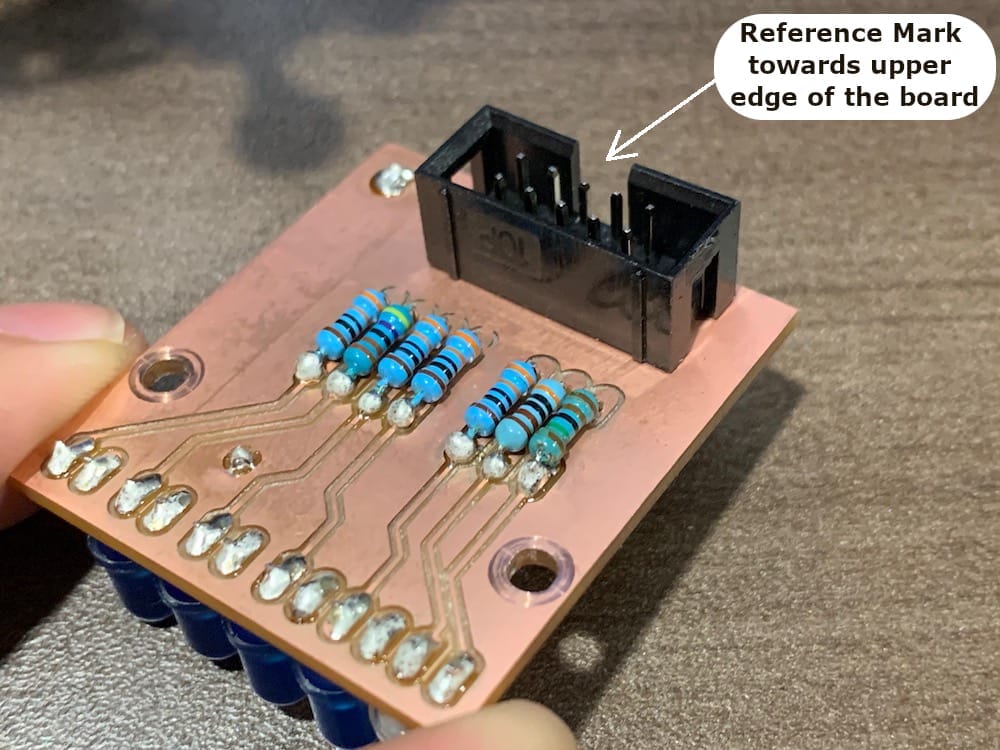
Fig 10.2-10. Populated LED Board
Some simple (optional) tests can be performed on the completed LED Board to ensure that the components have been installed and soldered correctly. A multimeter equipped with a Diode Test mode is required to perform the tests. The following figures illustrate where the positive (red) and ground (black) probes of the multimeter need to be positioned to perform the tests. The test is successful if the LED listed in the figures below turns on when the multimeter probes are connected.
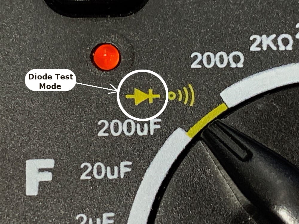
Fig 10.2-11. Diode Test Mode
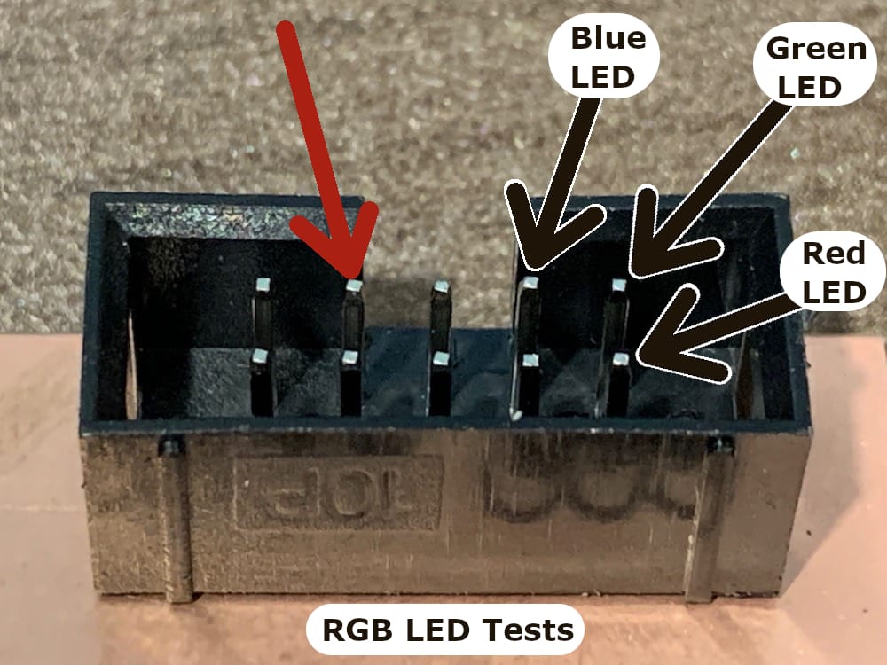
Fig 10.2-12. RGB LED Tests
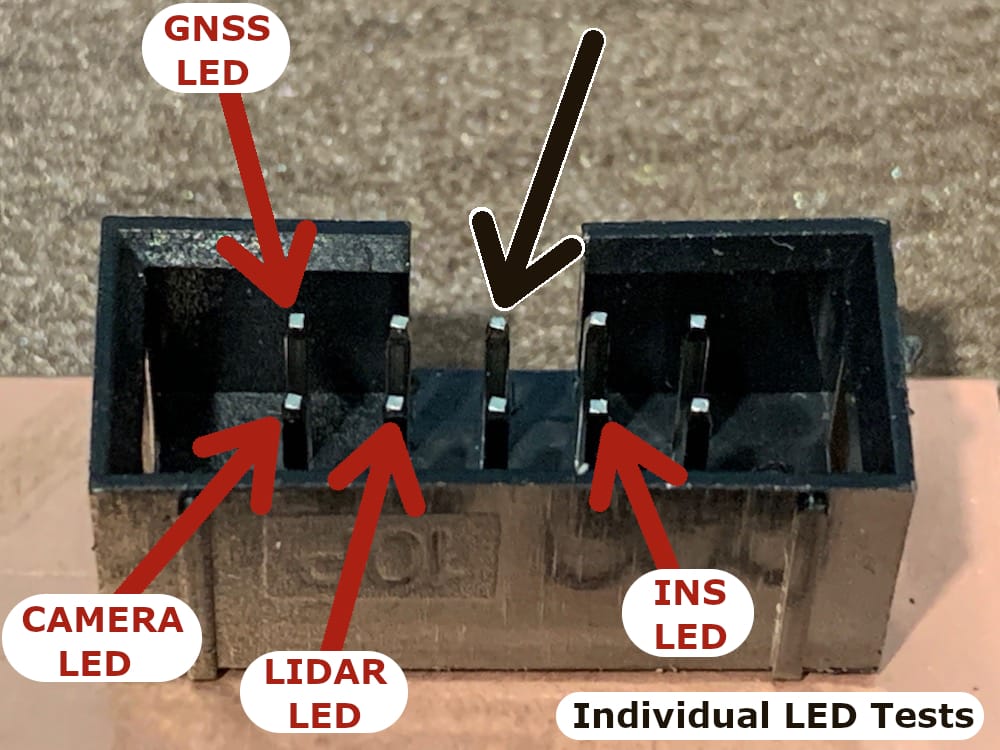
Fig 10.2-13. Indiv. LED Tests
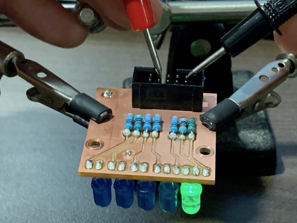
Fig 10.2-14. RGB - Green Test
Warning
DOUBLE AND TRIPLE CHECK YOUR SOLDERED CONNECTIONS AND MAKE SURE NO SHORT CIRCUITS, AND NO COLD SOLDERS EXIST!
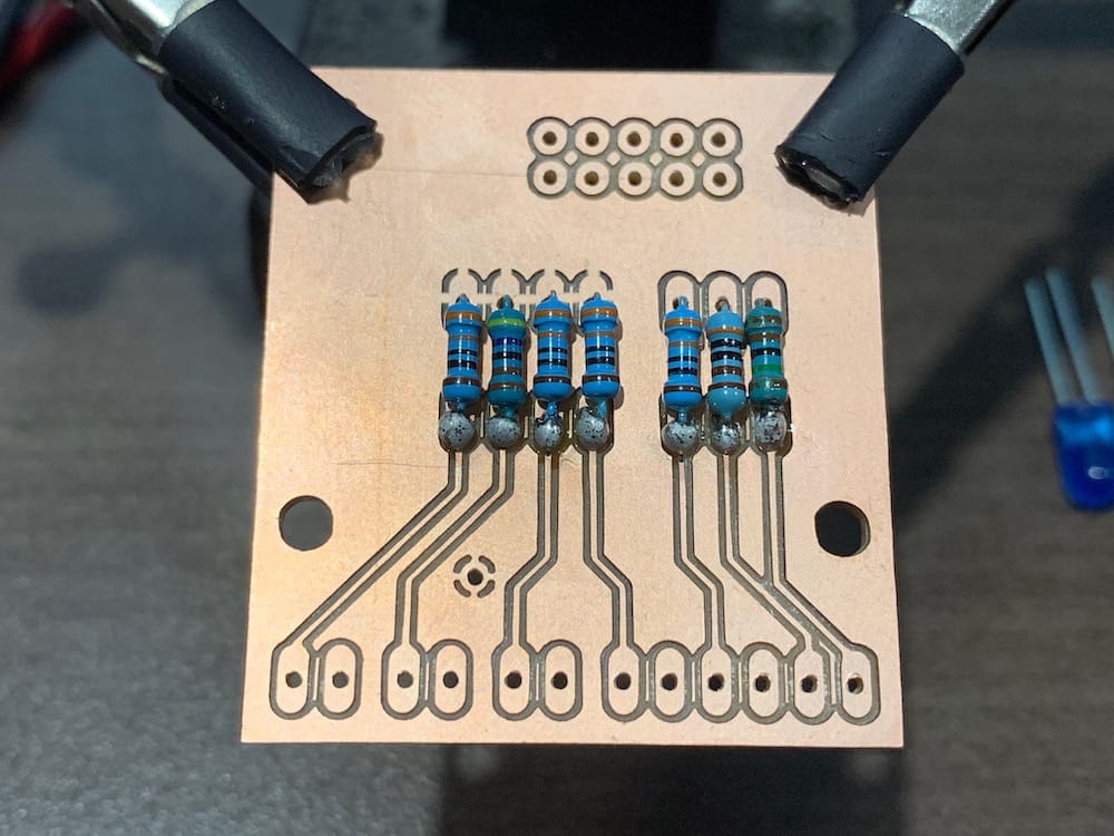
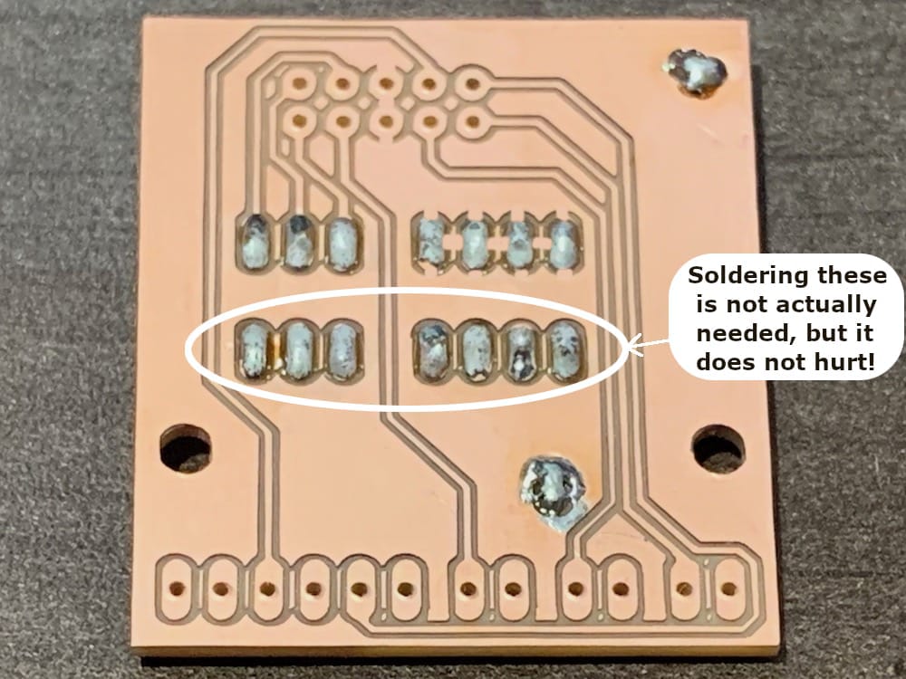
10.3. APX-18 Board
The following components are needed to assemble the OpenMMS APX-18 Board v1.3.
1 @ 2x5 ribbon cable jack
3 @ 1.0 Kohm through-hole resistors (1/4 Watt)
3 @ BC337 (or 2N2222) NPN transistors
1 @ Molex 936358314 ethernet jack with magnetics
1 @ 2-wire JST male connector 22 AWG cable
1 @ Samtec MMS-122-01-L-DV - 44-pin header
OpenMMS APX-18 Board v1.3
Header pins
Heat-shrink tubing
Excess wire for connecting vias (not shown)
Ferrite ring (optional, not shown)
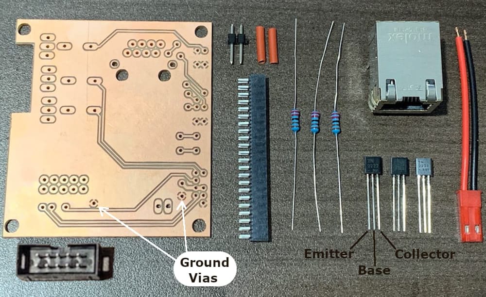
Fig 10.3-1. Components needed to assemble the APX-18 Board
Attention
The APX-18 requires clean 3.3V DC to operate. The tolerances for the power supply are specified as being between +5% (3.46V) and -3% (3.2V). Therefore, a high-quality lower gauge power cable should be used to connect the APX-18 Board to the RPi Board. The APX-18 will not properly boot-up if a voltage drop of more than 0.1V occurs along the power cable between the boards.
BE CAREFUL, NOT ALL 22AWG WIRE IS TRULY 22AWG!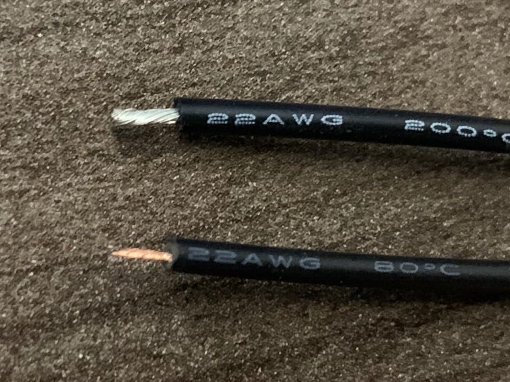
Fig 10.3-2. 22AWG wire differences
Begin by soldering wires to the top and bottom layers through the two ground plane vias and the twelve signal vias (see the figure below). Take your time soldering the signal vias as the soldering pads are relatively small, and the solder can easily bridge to the ground plane and create a potentially damaging short circuit. Next, installing the three resistors into their respective holes in the top layer. The right side of each resistor needs to be soldered on the top layer. Insert the three NPN transistors into their respective holes in the top layer. The transistors have polarity and need to be inserted correctly within the board (see the figure below). Flip the board over and solder the resistors and transistor connections to the bottom layer.
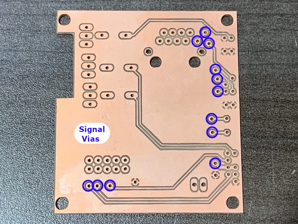
Fig 10.3-3. 12 signal vias to solder (ON BOTH LAYERS)
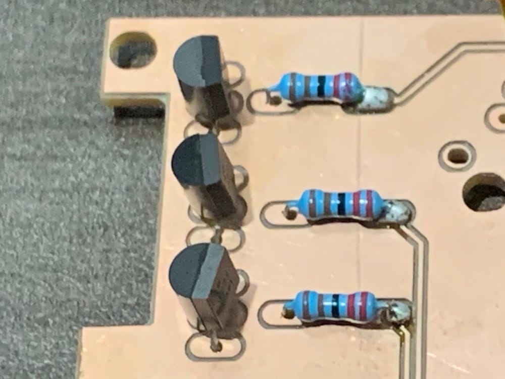
Fig 10.3-4. Transistors and resistors installed
Next, cut the 2-wire JST connector cable to an overall length of 6cm OR, optionally cut it to a length of 15cm and wrap the cable as many times as possible around a ferrite ring. If the ferrite ring does not have a protective non-conductive coating on it, make sure to cover the ring after wrapping the wire around it. Slide a piece of heat-shrink tubing, ideally with a unique color, over both wires. As there are several wires inside the OpenMMS case with the same connector type, the unique color heat-shrink tubing is used to simplify assembling the sensor later on. Next, solder each wire to a block of two header pins and ensure heat-shrink tubing is used to insulate the wires. Insert the 2-wire JST connector cable into the top layer of the APX-18 Board, as shown below, and solder it to the bottom layer.
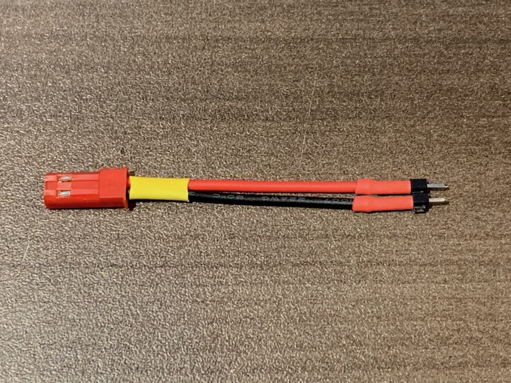
Fig 10.3-5. 2-wire JST on header pins
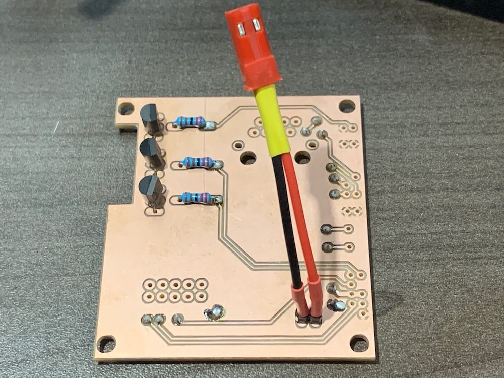
Fig 10.3-6. 2-wire JST installed
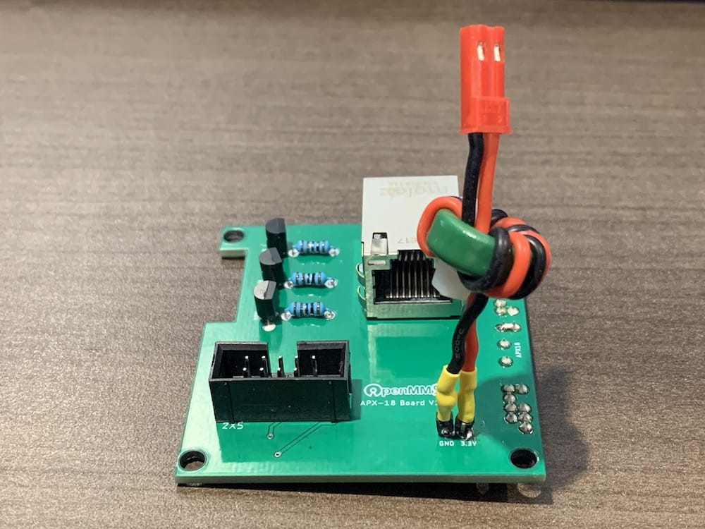
Fig 10.3-7. 2-wire JST with ferrite ring
Next, the 44-pin header that connects to the Applanix APX-18 sensor needs to be modified. To make more room on the PCB and allow for traces to be routed easier, the unused pins from the header need to be manually removed. Removing the unused pins can be accomplished using a small set of pliers and simply pulling the individual pins out of the header. This process is non-destructive, so if a mistake is made, the pin can be re-inserted back into the header. The header is installed on the bottom layer and therefore soldered to the top layer. View the figure below to determine which header pins need to be removed. Once the header fits properly into the board, solder it in place. Next, the ethernet jack needs to have four pins snipped from the bottom of it. Once these pins have been removed, the ethernet jack can be installed into the top layer. The 2x5 ribbon cable jack can also be installed into the top layer, pay close attention to the orientation of the jack’s reference mark.
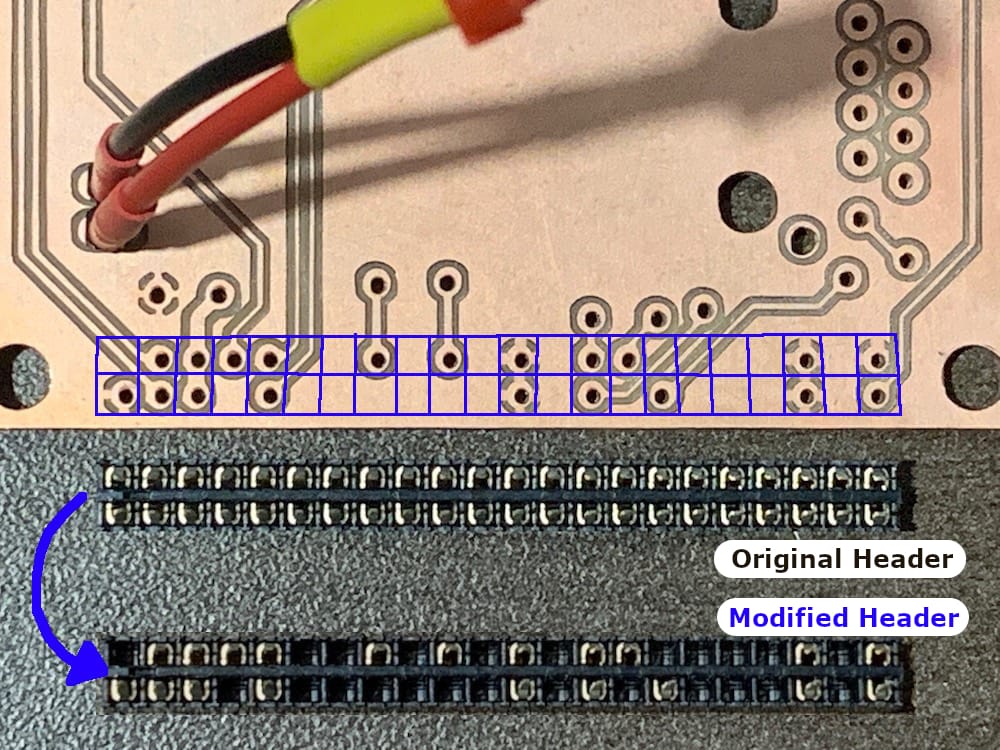
Fig 10.3-8. Modified 44-pin header
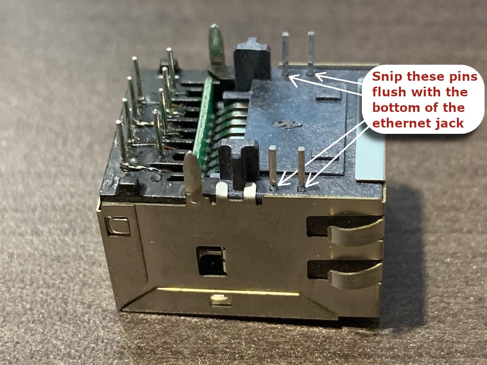
Fig 10.3-9. Ethernet jack pins to snip
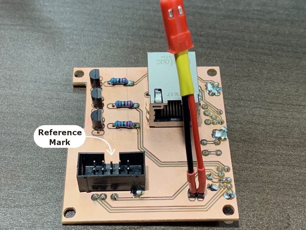
Fig 10.3-10. Populated APX-18 Board
Warning
DOUBLE AND TRIPLE CHECK YOUR SOLDERED CONNECTIONS AND MAKE SURE NO SHORT CIRCUITS, AND NO COLD SOLDERS EXIST!
10.4. RPi Board
The following components are needed to assemble the OpenMMS RPi Board v1.3.
3 @ 2x5 ribbon cable jack
2 @ 330 ohm through-hole resistor (1/4 Watt)
3 @ 680 ohm through-hole resistor (1/4 Watt)
1 @ 1.5 Kohm through-hole resistor (1/4 Watt)
2 @ 2.2 Kohm through-hole resistor (1/4 Watt)
1 @ 10 Kohm through-hole resistor (1/4 Watt)
1 @ 33 Kohm through-hole resistor (1/4 Watt)
3 @ BC337 (or 2N2222) NPN transistor
1 @ 0.33 uF ceramic capacitor
1 @ 10 uF ceramic capacitor
2 @ 22 uF ceramic capacitor
1 @ 1N4001G diode
3.3V regulator (CUI V7803-2000)
9V Low Drop Out regulator (Rohm BA90JC5)
Assmann A-2004-2-4-R ethernet jack
SPDT relay (JZC-11F)
Mini-fuse holder (Littelfuse 01530007Z) with fuse
8-wire screw terminal (Phoenix Contact 1725711)
Raspberry Pi 40-pin stacking header
Preconfigured Adafruit Pro Trinket
OpenMMS RPi Board v1.3
MicroUSB power cable (included with Hak5 ethernet switch)
2 @ JR/Futaba 3-wire cable with male connector 22-26AWG
1 @ JR/Futaba 2-wire cable with male connector 22-26AWG
1 @ JR/Futaba 2-wire cable with female connector 22-26AWG
2 @ JST 2-wire cable with male connector 22AWG
3 @ JST 2-wire cable with female connector 22AWG
Header pins
Heat-shrink tubing
Excess wire for connecting vias (not shown)
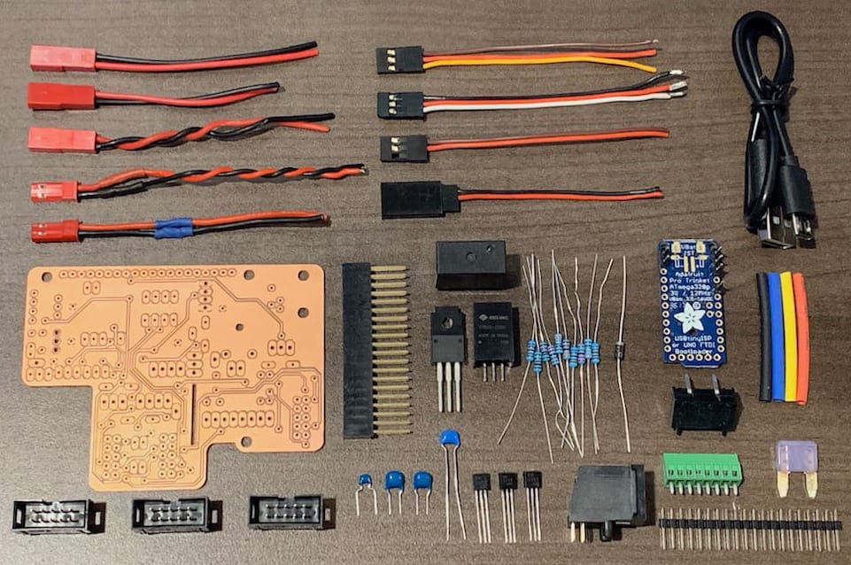
Fig 10.4-1. Components needed to assemble the RPi Board
Warning
The RPi Board circuitry is much more complicated than the previous OpenMMS PCBs. As a result, it is STRONGLY RECOMMENDED to be testing the soldered connections immediately after completing them to ensure no short circuits or bridged connections exist. NO EXHAUSTIVE BOARD TEST PROCEDURES ARE INCLUDED AFTER ASSEMBLY IS COMPLETE.
Begin by soldering wires to the top and bottom layers through the ten ground vias, as shown in figure 10.4-2. There are a total of forty-seven signal vias that need to be soldered before the board can be populated with its components. It is recommended to take a systematic approach to solder all the signal vias to avoid missing any of them. The RPi Board can be divided into three arbitrary sections that each have a similar number of signal vias within them. Start by soldering the four ‘boundary’ vias, as shown in figure 10.4-3, as these vias are used to demarcate the sections.
Next, examine each of the figures below, and complete the soldering for the vias within each section. DO NOT FORGET THAT VIAS REQUIRE SOLDERING ON BOTH THE TOP LAYER AND THE BOTTOM LAYER. Soldering the vias is a tedious task, but a vital one!
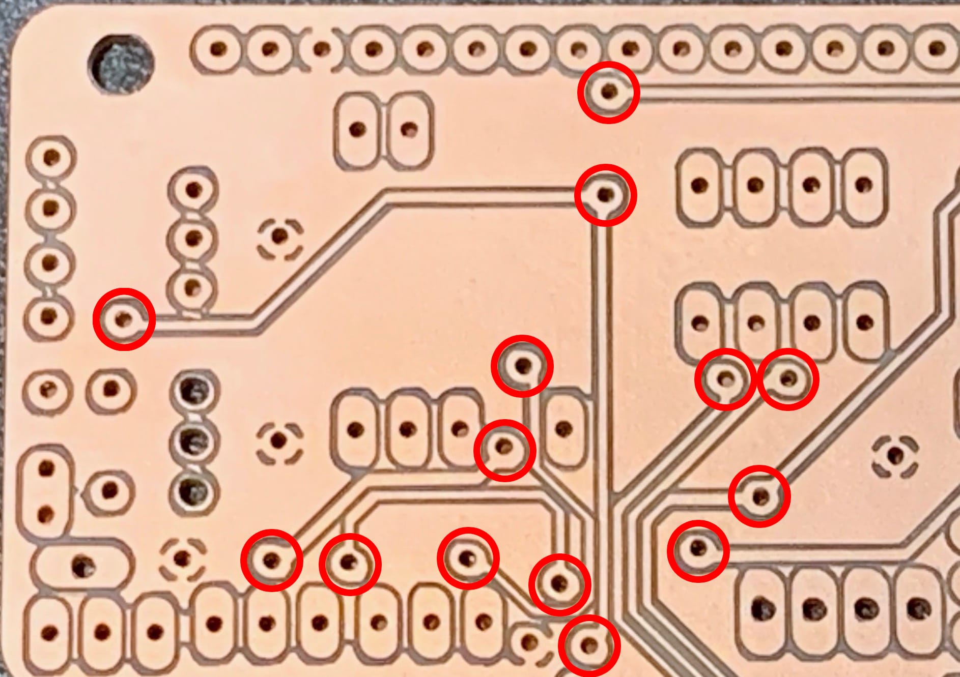
Fig 10.4-4. Red section (14 vias)
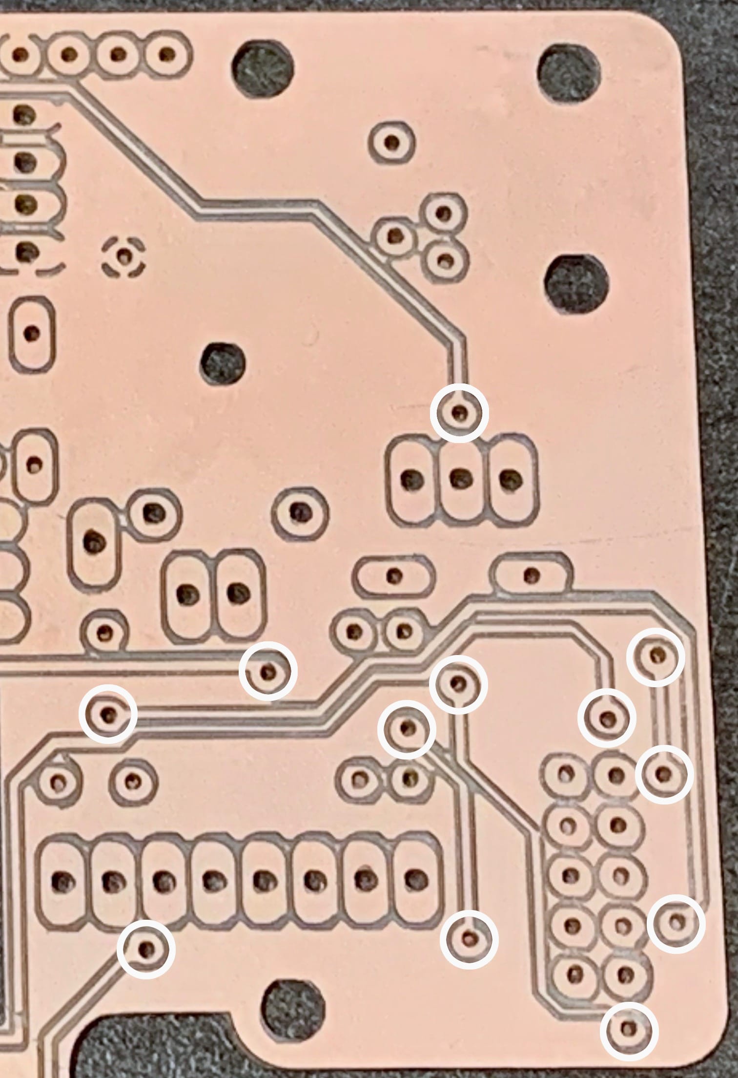
Fig 10.4-5. White section (12 vias)
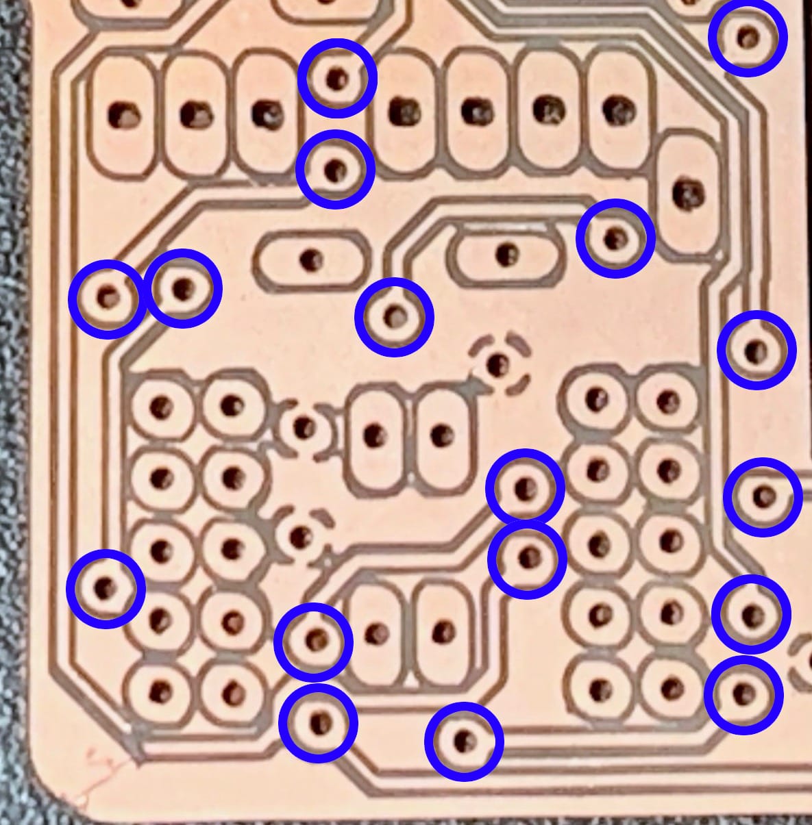
Fig 10.4-6. Blue section (17 vias)
Install the ten resistors into their respective holes on the top layer of PCB. Resistors do not have polarity, so it does not matter which end goes where. Refer to the RPi Bantam - interactive PCB viewer in section 5.6 for details on which resistor goes where. Solder the resistors to the bottom layer. Install the 3.3V and 9V regulators and their respective ceramic capacitors into their holes on the top layer. Ceramic capacitors do not have polarity, so they can be installed in any orientation. Lastly, install the three NPN transistors into the top layer of the RPi Board.
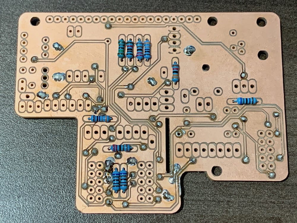
Fig 10.4-7. Ten resistors installed
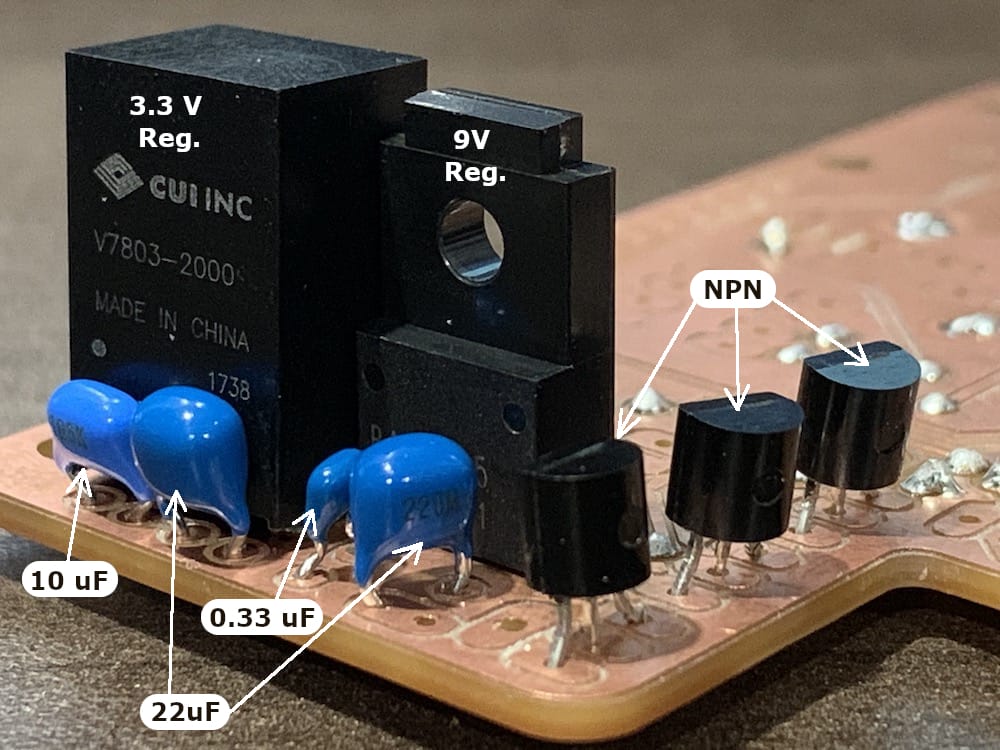
Fig 10.4-8. Voltage regulators, capacitors and transistors installed
Next, the mechanical relay, diode, and 8-wire screw terminal can be installed in the top layer. The relay only fits into the PCB holes one way. The diode does have polarity, so examine the figures below to understand its correct orientation with respect to its grey colored band. When installing the screw terminal block, be sure the openings are facing the outside edge of the RPi Board.
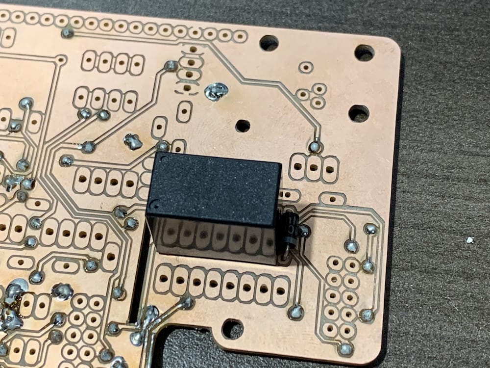
Fig 10.4-9. Relay and diode installed
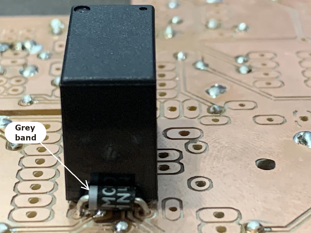
Fig 10.4-10. Diode orientation details
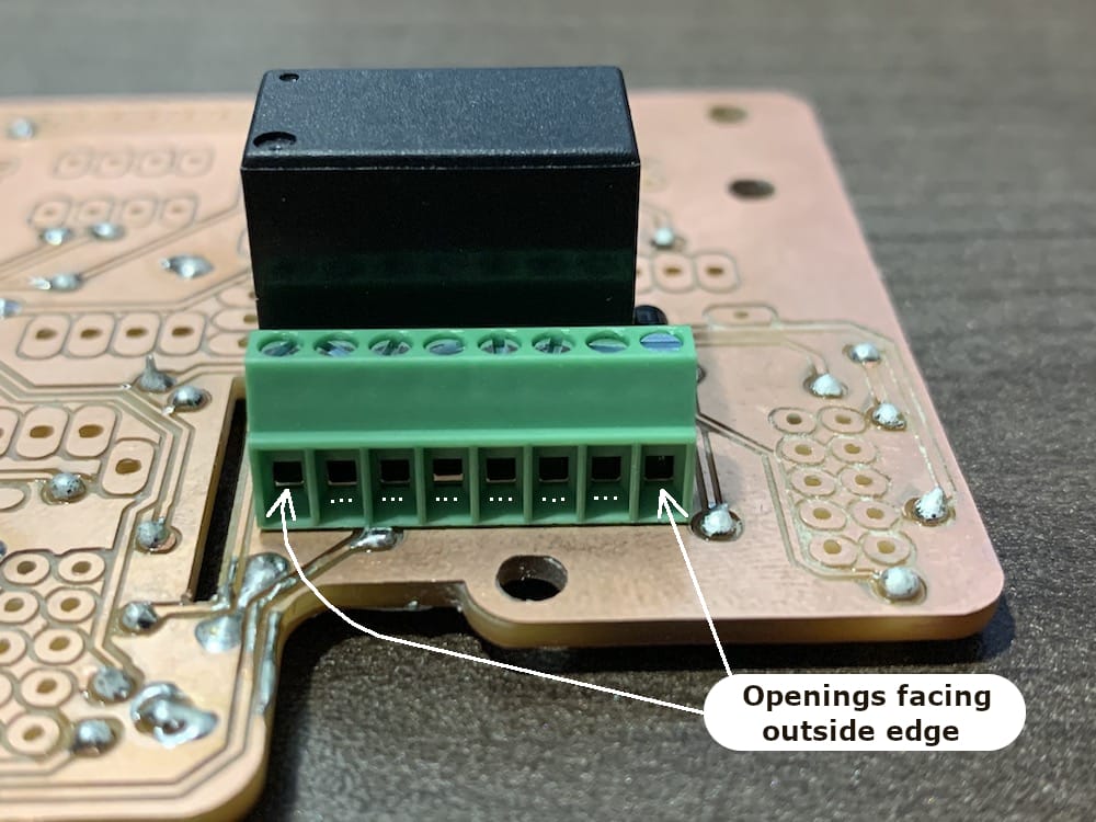
Fig 10.4-11. Screw terminal installed
Next, the ethernet jack and mini-fuse holder can be installed in the top layer. Before the ethernet jack can be installed into the board, four pins on the bottom of the jack must be removed (see the figure below). The mini-fuse holder needs to be installed, so the fuse is pointing towards the upper edge of the board. Both of these components have plastic mounting tabs that need to be friction fit into the support holes on the RPi Board. Slowly and evenly apply pressure when installing these components until they are fully seated on the board.
Attention
It is recommended to use, at a maximum, a 3A mini-fuse.
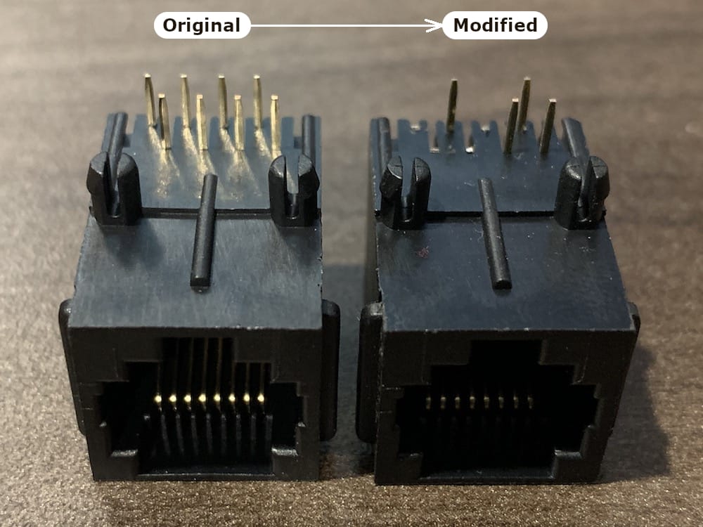
Fig 10.4-12. Ethernet jack pins to remove
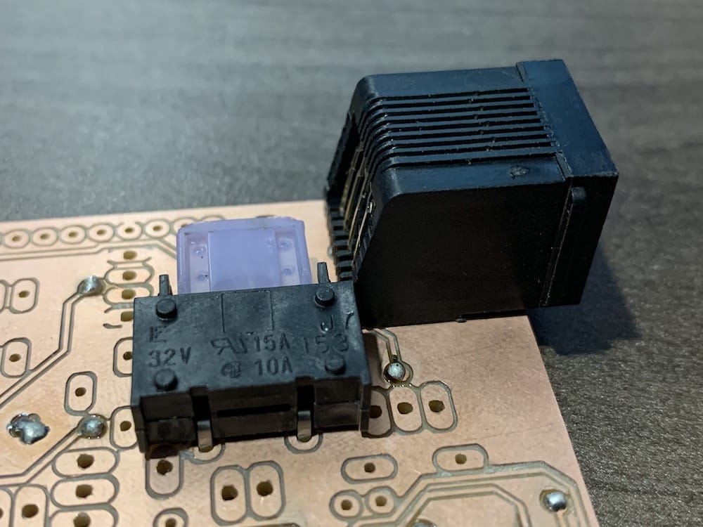
Fig 10.4-13. Ethernet jack and mini-fuse holder installed
Next, the three 2x5 ribbon cable jacks and the Adafruit Pro Trinket components can be installed. Pay close attention to the orientation of the 2x5 jacks, notice that one is installed in a different orientation than the other two. As mentioned in section 8.3, the Arduino Intervalometer Sketch should be installed (and tested) on the Pro Trinket before the component is soldered onto the RPi Board.
The next step requires using the Raspberry Pi 4 Model B computer to ensure the 40-pin stacking header component is in the proper position before being soldered to the RPi Board. Affix three 20mm standoffs to the Raspberry Pi computer’s mounting holes (see figure below). Only the row of General Purpose Input Output (GPIO) pins adjacent to the computer’s outside edge are used, so the twenty stacking pins on the inside row of the header need to be manually removed. Use a small set of pliers to grab each pin and remove it from the header (see figure below).
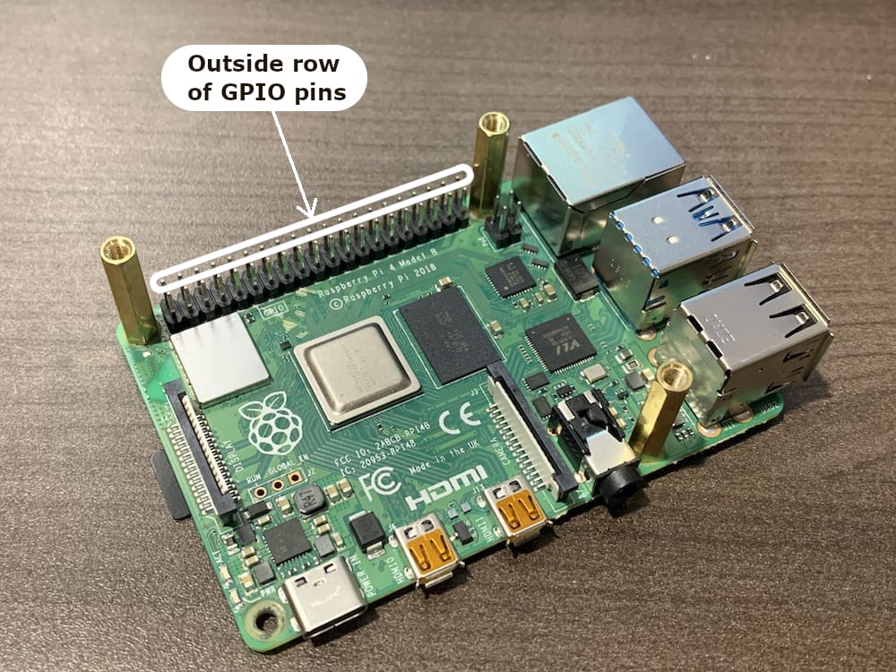
Fig 10.4-16. Raspberry Pi computer with standoffs installed

Fig 10.4-17. Inside row of stacking header pins removed
Next, install the stacking header onto the GPIO pins of the Raspberry Pi computer. Align the twenty stacking pins with the holes in the bottom layer of the RPI Board, and then, install three M3 button-head bolts into the standoffs to temporarily hold the RPi Board in the correct position. The stacking header pins are likely just visible through their holes on the top layer of the RPi Board. However, this is not a concern because the stacking header pins need to be soldered on the bottom layer of the RPi Board. Flip the RPi Board and Raspberry Pi computer over so the RPi Board is on the bottom. Solder only the first and the last stacking pin to their respective pads on the bottom layer of the RPi Board. Remove the button-head bolts holding the board and the computer together. Detach the RPi Board from the computer and complete the remaining solder connections for installing the stacking header onto the RPi Board.
Lastly, ten cables must be soldered to blocks of header pins before being soldered onto the RPi Board. As discussed in the APX-18 PCB assembly section, uniquely colored heat-shrink tubing is applied to the end of each cable to ID the cable. Two cables are made shorter than the others, rather than having a unique color ID. The ideal length for each cable is approximately 8cm, except for the micro-USB cable, which should be about 16cm. Be sure to use heat-shrink tubing to insulate the soldered connections. The following figure illustrates the cables that need to be prepared.
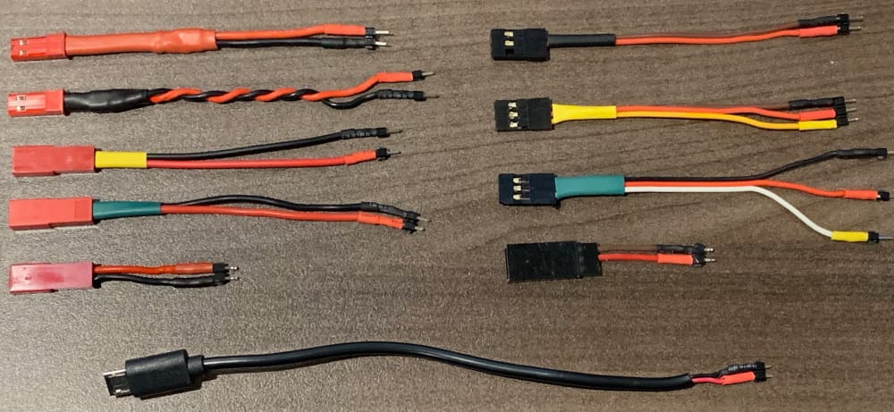
Fig 10.4-20. Cables for the RPi Board
The following nine figures illustrate where the ten cables need to be inserted within the top layer of the RPi Board. After inserting each cable, it needs to be soldered to the bottom layer of the RPi Board. Pay close attention to where the individual header pin for each wire is installed, as damage could result if the cables are installed incorrectly.
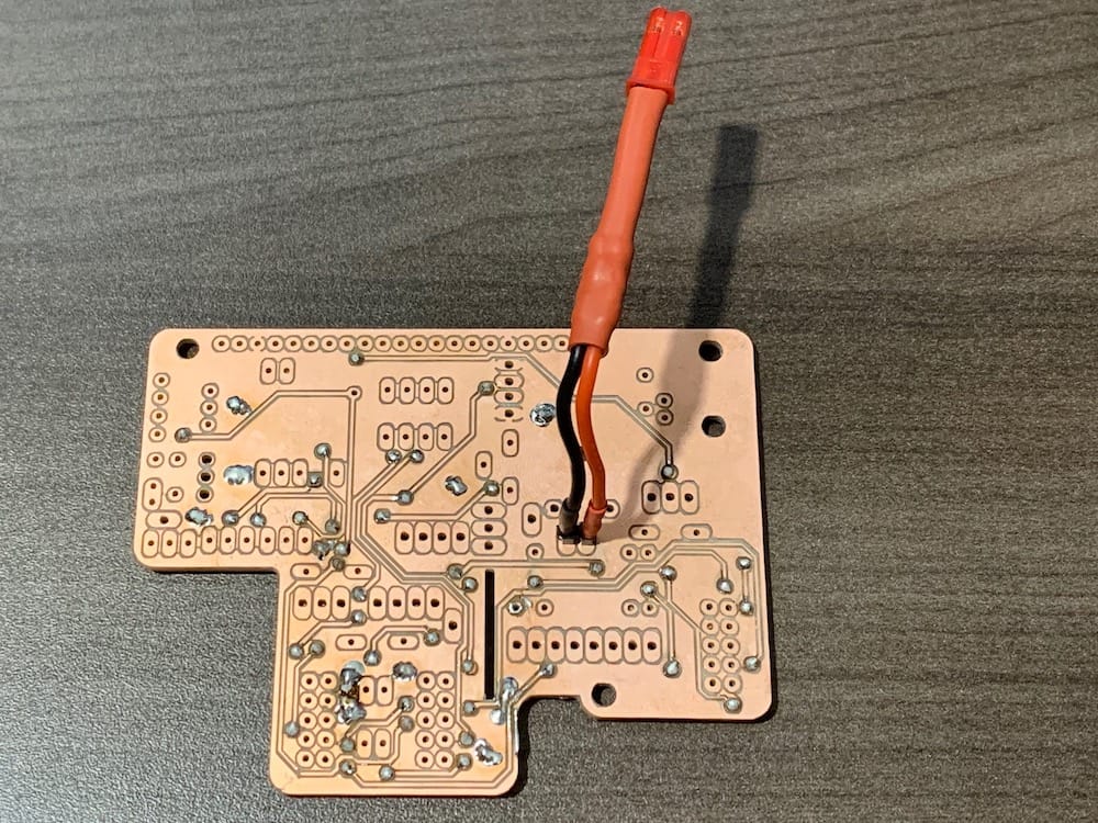
Fig 10.4-21. Cable to external power
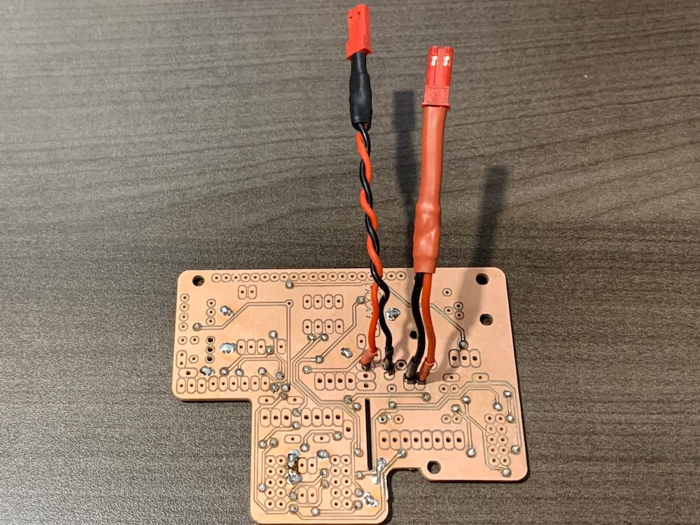
Fig 10.4-22. Cable to power pushbutton
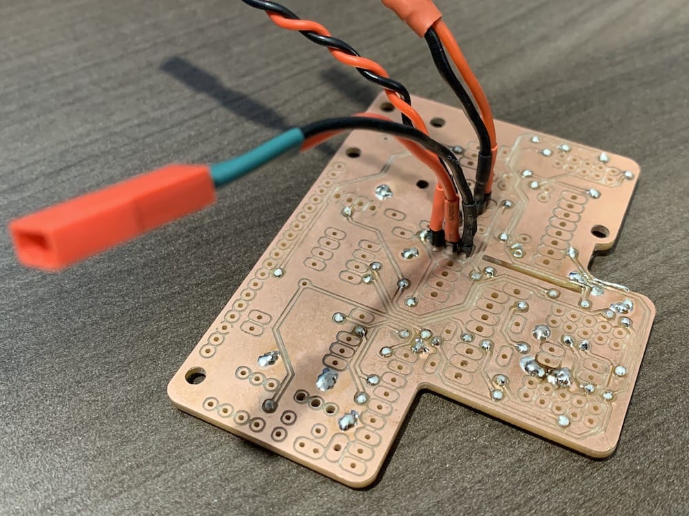
Fig 10.4-23. Cable to UBEC Duo input
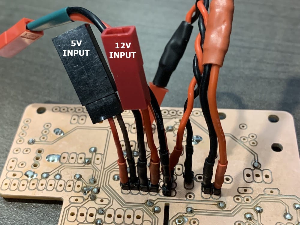
Fig 10.4-24. Cables to UBEC Duo outputs
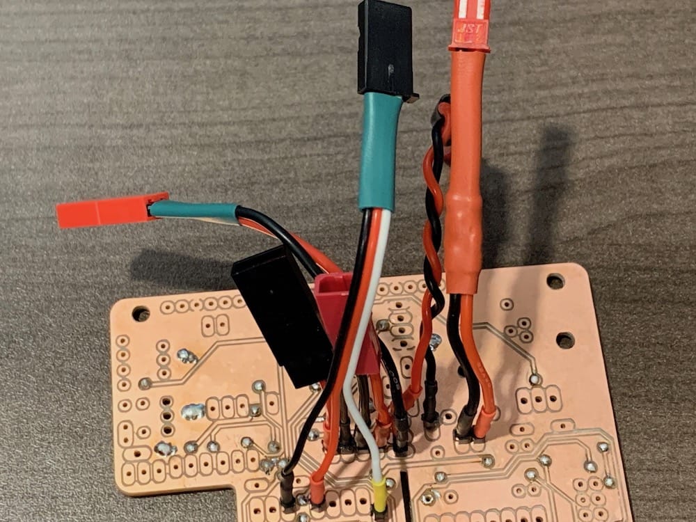
Fig 10.4-25. Cable to camera event port
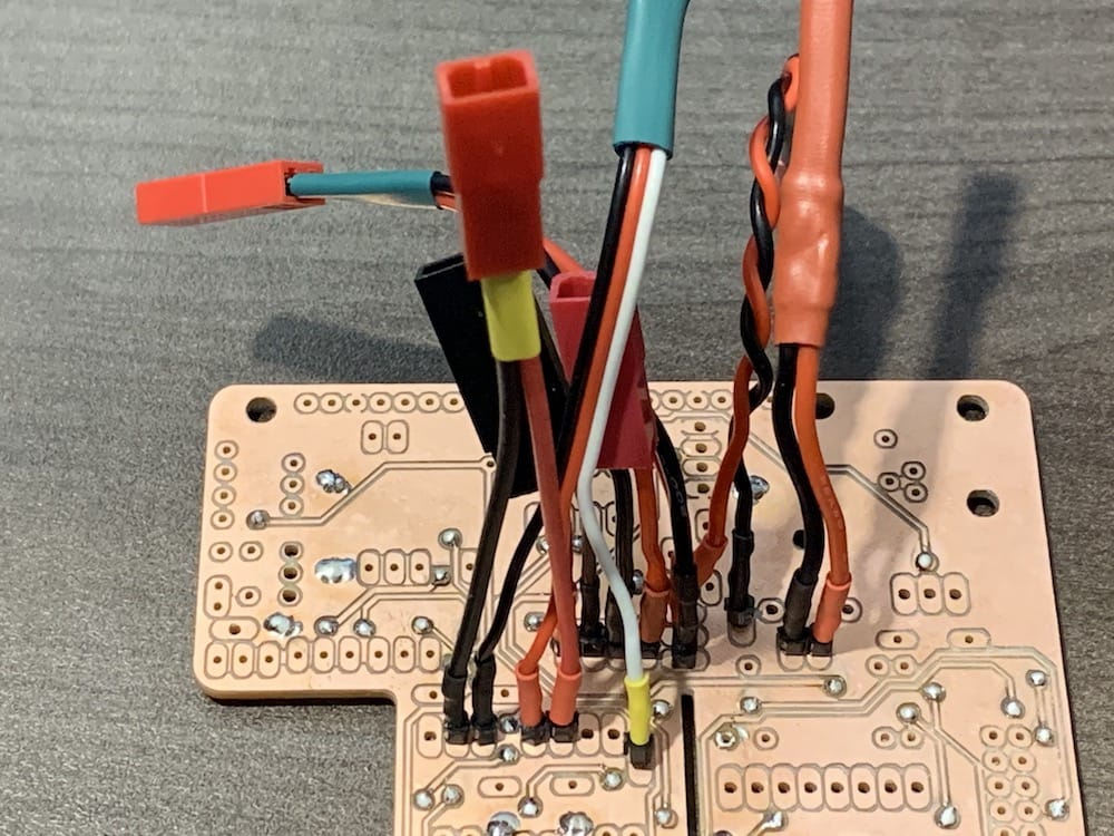
Fig 10.4-26. Cable to APX-18 Board
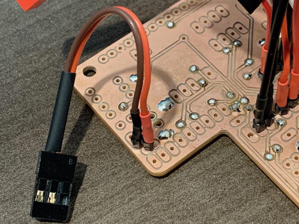
Fig 10.4-27. Cable to camera power port
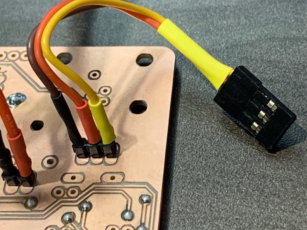
Fig 10.4-28. Cable to input pushbutton
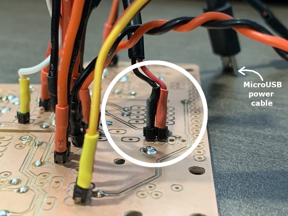
Fig 10.4-29. Micro-USB to ethernet switch
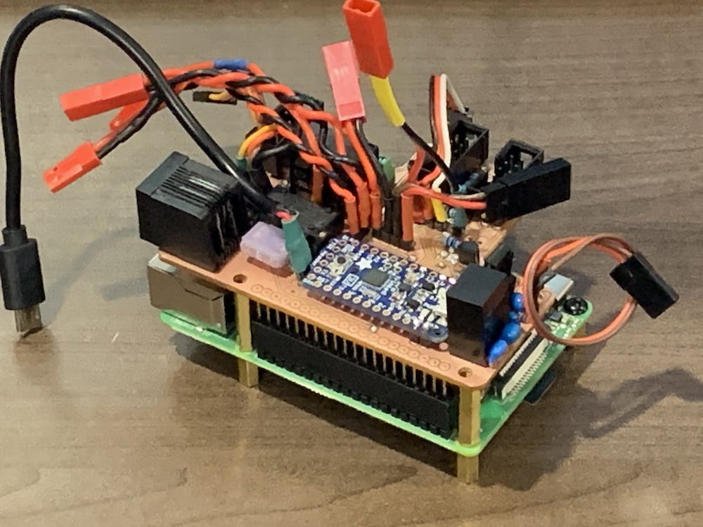
Fig 10.4-30. Populated RPi Board
Warning
DOUBLE AND TRIPLE CHECK YOUR SOLDERED CONNECTIONS AND MAKE SURE NO SHORT CIRCUITS, AND NO COLD SOLDERS EXIST!
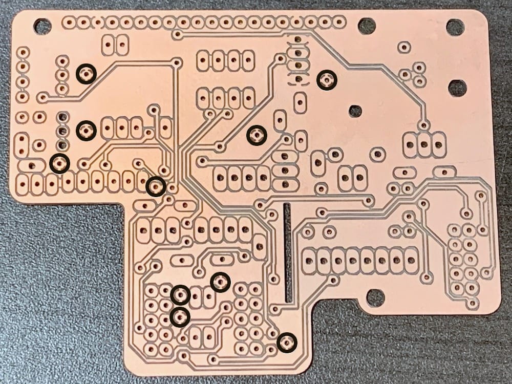
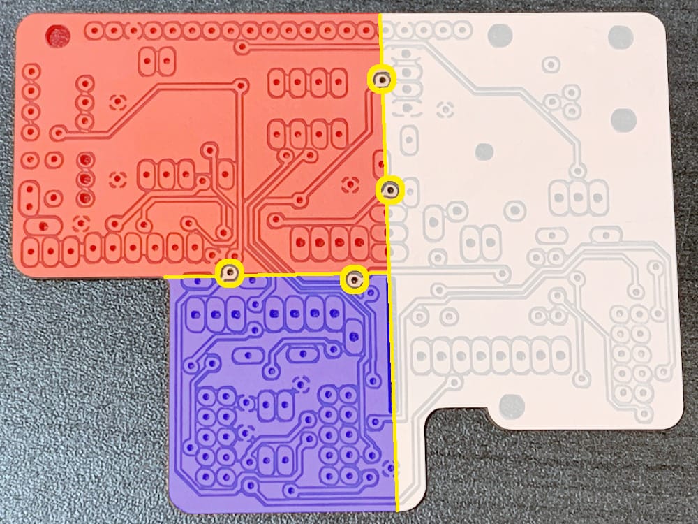
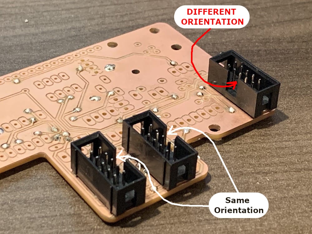
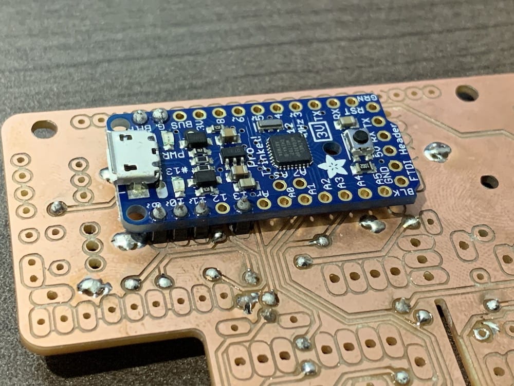
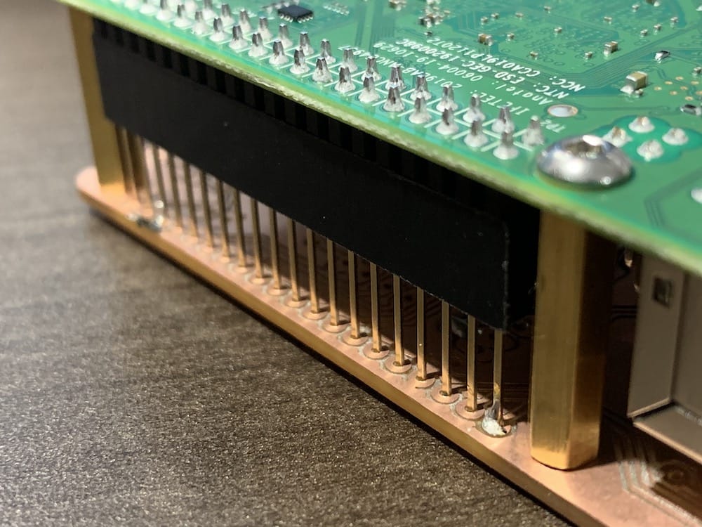
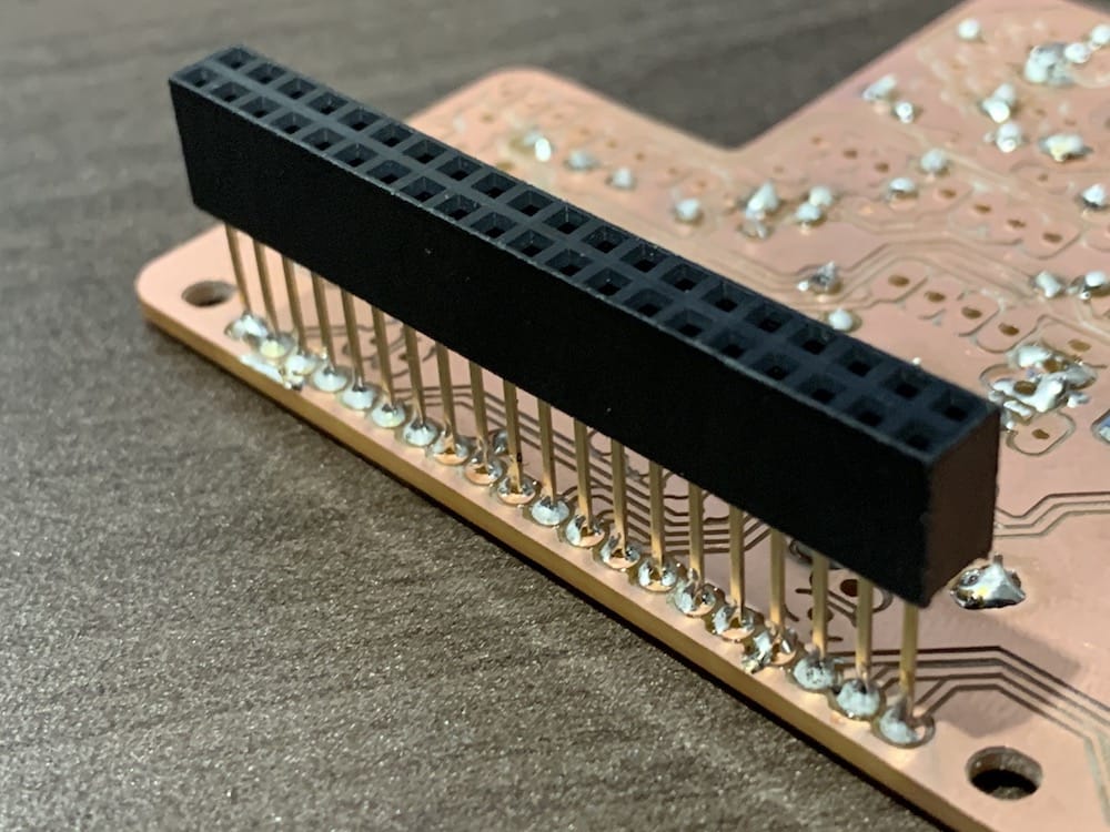
CONGRATULATIONS!
YOU HAVE NOW FINISHED ASSEMBLING ALL THE PRINTED CIRCUIT BOARDS! THAT WAS A BIG TASK!
11. Aluminum Parts Assembly
Important
When installing any bolt into/through a threaded hole (inside or outside the case), it is STRONGLY RECOMMENDED that regular (medium strength), non-conductive Loctite be applied to the bolt. Within the instructions below, the use of Loctite is not mentioned only because of the instruction’s redundancy.
A 2.0mm Hex/Allen driver is traditionally used to tighten 3mm metric (M3) button-head bolts. However, from the author’s experience, it is STRONGLY RECOMMENDED to use a Torx 8 (T8) driver instead of the 2.0mm Hex driver. If an M3 button-head bolt becomes ‘stripped’, and neither the 2.0mm Hex nor Torx 8 driver can provide adequate ‘grip’ on the head of the bolt, attempt to use a Torx 9 (T9) driver on the bolt.
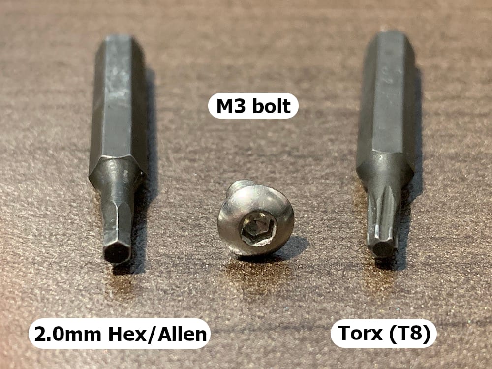
Fig 11.0-1. Driver options for working with M3 bolts
11.1. Overview
Each of the six faces of the case is first installed with all their respective hardware components, sensors, etc., and then the faces are assembled to create the finished sensor. Once again, the order of operations to follow is critical! Pay close attention to the instructions!!
11.2. Top Face Assembly
The following components are needed to assemble the top face of the OpenMMS case.
2 @ 3mm (M3) button-head bolts, 12mm in length with Nyloc nuts
4 @ 4mm (M4) hex bolts, ~16mm in length with Nyloc nuts
OpenMMS Left and Right reinforcing brackets
22 AWG 2-pin JST power connector, 15cm in length
Heat-shrink tubing
XT-60 female housing/male pin connector
OpenMMS top face
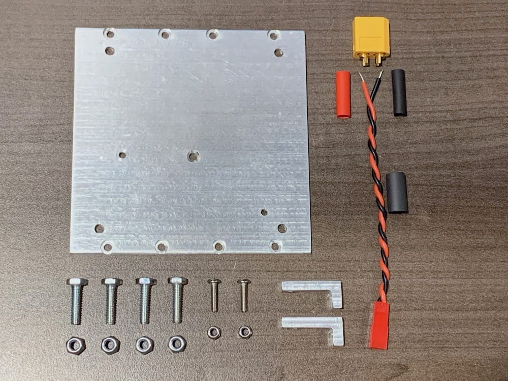
Fig 11.2-1. Components needed to assemble the top face
Start by affixing a piece of heat-shrink tubing at the approximate midpoint of the 22 AWG wire. Next, carefully pass the wire through the hole near the center of the top face, stopping when the heat-shrink tubing is seen equally on both sides. Solder an XT-60 female housing/male pin connector to the unpopulated side of the 22 AWG wire (BEING VERY CAREFUL TO ENSURE THE POLARITY OF THE XT-60 CONNECTOR MATCHES THAT OF THE JST CONNECTOR). Next, insert the M4 16mm long hex bolts, from the inside of top face, through the larger holes near the corners of the front face. Thread and completely tighten a Nyloc nut onto each of the bolts. Lastly, insert a 12mm long M3 bolt into the two smaller holes, from the outside of the top face, and thread them into the Left and Right reinforcing brackets. Position a Nyloc nut on the bottom of each reinforcing bracket and thread the M3 bolts through the brackets and the Nyloc nuts. After tightening the M3 bolt, a wrench can be used to tighten the Nyloc nut. Try to ensure the reinforcing brackets are perpendicular to the outside edges of the top face.
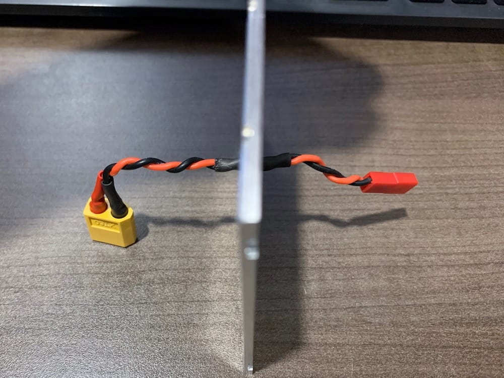
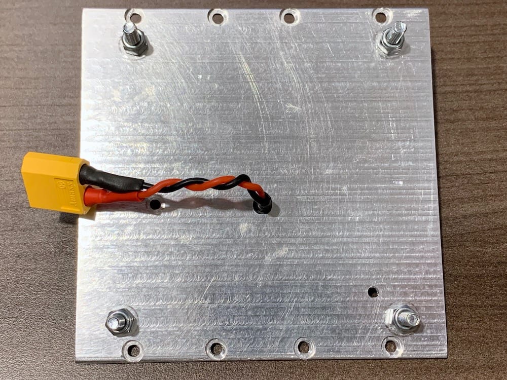
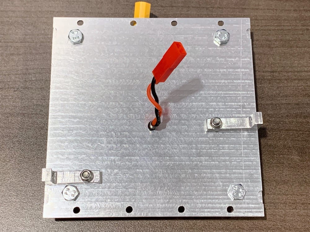
11.3. Bottom Face Assembly
DISCLAIMER
In this step, the expensive and sensitive Applanix APX-18 GNSS-INS sensor is used. THE READER IS RESPONSIBLE FOR ALL THE RISKS ASSOCIATED WITH THE HANDLING AND USE OF THE APPLANIX APX-18 SENSOR!
The following components are needed to assemble the bottom face of the OpenMMS case.
10 @ 3mm (M3) button-head bolts, 5mm in length
8 @ 3mm (M3) flat washers
6 @ 3mm (M3) button-head bolts, 10mm in length
4 @ 3mm (M3) Male/Female standoffs, 6mm in length
6 @ 3mm (M3) Female/Female standoffs, 15mm in length
Raspberry Pi Camera V2.1
Assembled OpenMMS APX-18 Board V1.3
OpenMMS bottom face
Applanix APX-18 GNSS-INS sensor
Kapton/Polyimide Tape (optional)
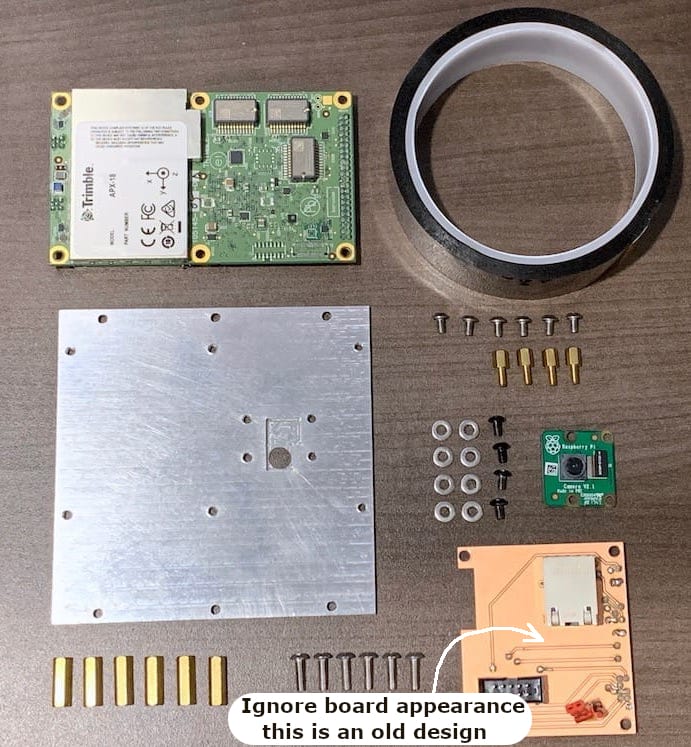
Fig 11.3-1. Components needed to assemble the bottom face
INFORMATION
The author of this documentation begins assembling the bottom face by wrapping Kapton tape around the exposed electronics on the right side of the Applanix APX-18 sensor. This instruction has NOT been approved by Applanix and therefore is NOT an OpenMMS assembly instruction.
The Raspberry Pi Camera V2.1 needs to have the four mounting holes carefully widen to allow for M3 bolts to be used to install the camera. The camera board is originally designed for 2mm (M2) bolts, so the holes need to be substantially widened. It is recommended to protect the exposed electronics on the Raspberry Pi Camera by using tape to cover them. Then using the Proxxon Drill Press with a 3/32” drill bit, very carefully and slowly drill through the four mounting holes on the camera board. Next, stack two M3 flat washers on top of each other and position them over each of the four holes surrounding the bottom face’s camera recess area. Gently insert the Raspberry Pi Camera into the recess area on the bottom face and secure it using four 5mm long M3 bolts. While tightening the bolts, be sure to apply even pressure across the camera board, or it may risk breaking. Next, thread and tighten the six 10mm long M3 bolts through the threaded holes in the bottom face, from the outside. On the inside of the bottom face, thread and tighten the six 15mm long M3 Female/Female standoffs onto the extruding M3 bolts.
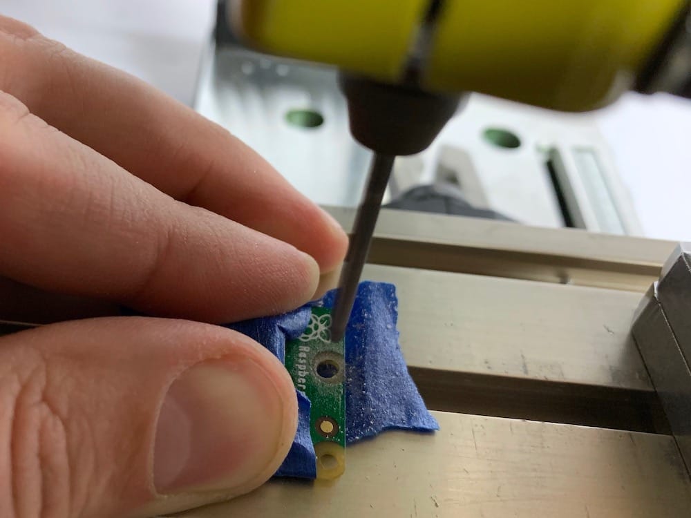
Fig 11.3-2. Widening Raspberry Pi Camera holes
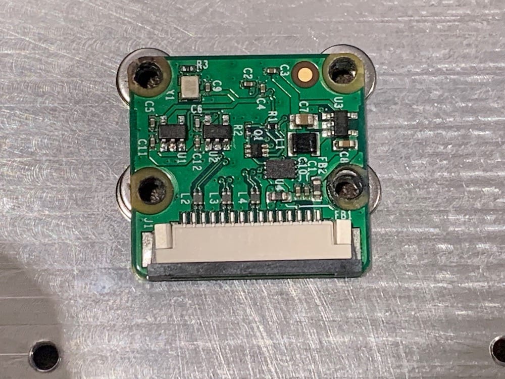
Fig 11.3-3. Double flat washers under camera board
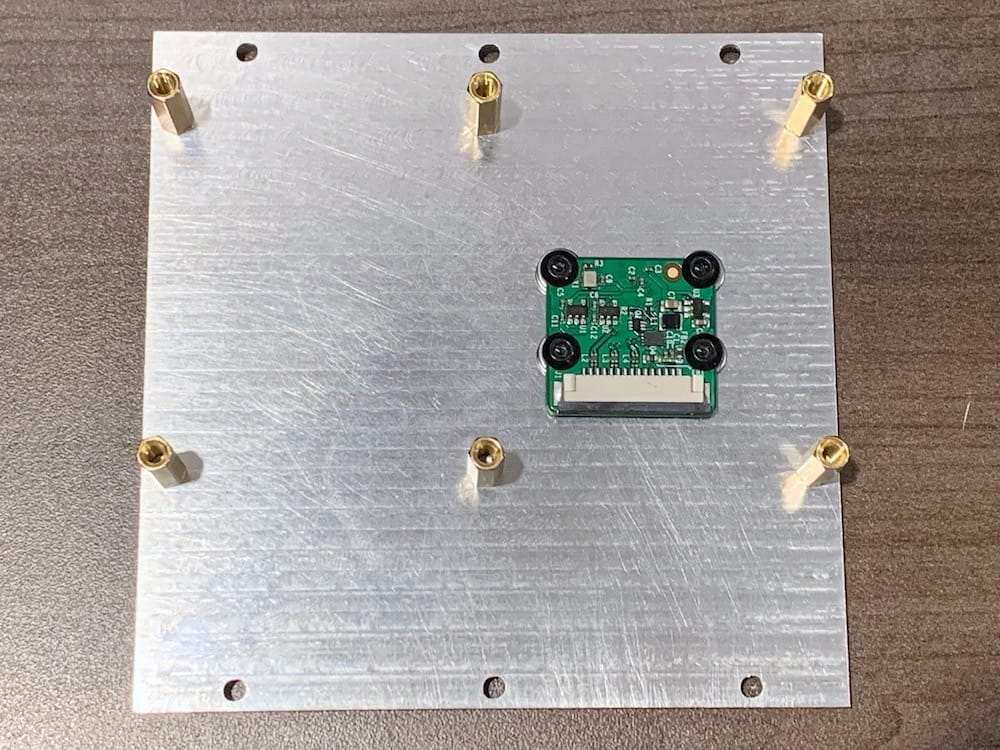
Fig 11.3-4. 15mm standoffs installed
Next, position the APX-18 sensor over the six standoffs and ensure that the sensor’s bottom side is evenly resting on all six standoffs. Secure the two left mounting holes using 5mm long M3 bolts and the center two and right two mounting holes using 6mm long Male/Female M3 standoffs. Be sure to evenly tighten the bolts and standoffs securing the APX-18 sensor, a little at a time. Lastly, install the OpenMMS APX-18 Board V1.3 onto the 44-pin header of the APX-18 sensor and secure it using four 5mm long M3 bolts.
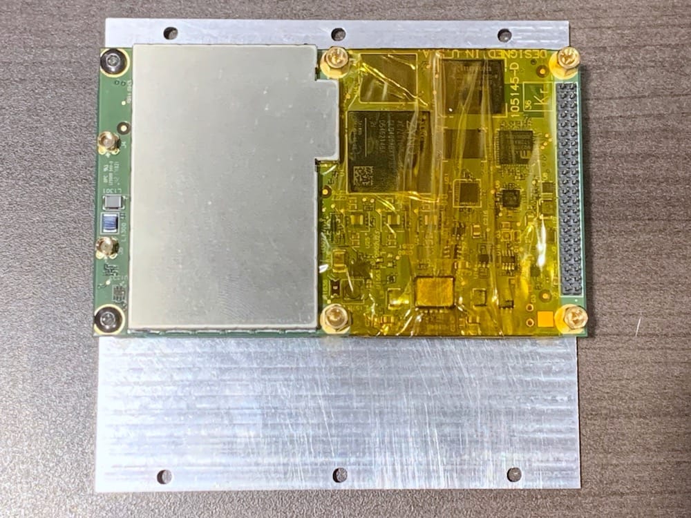
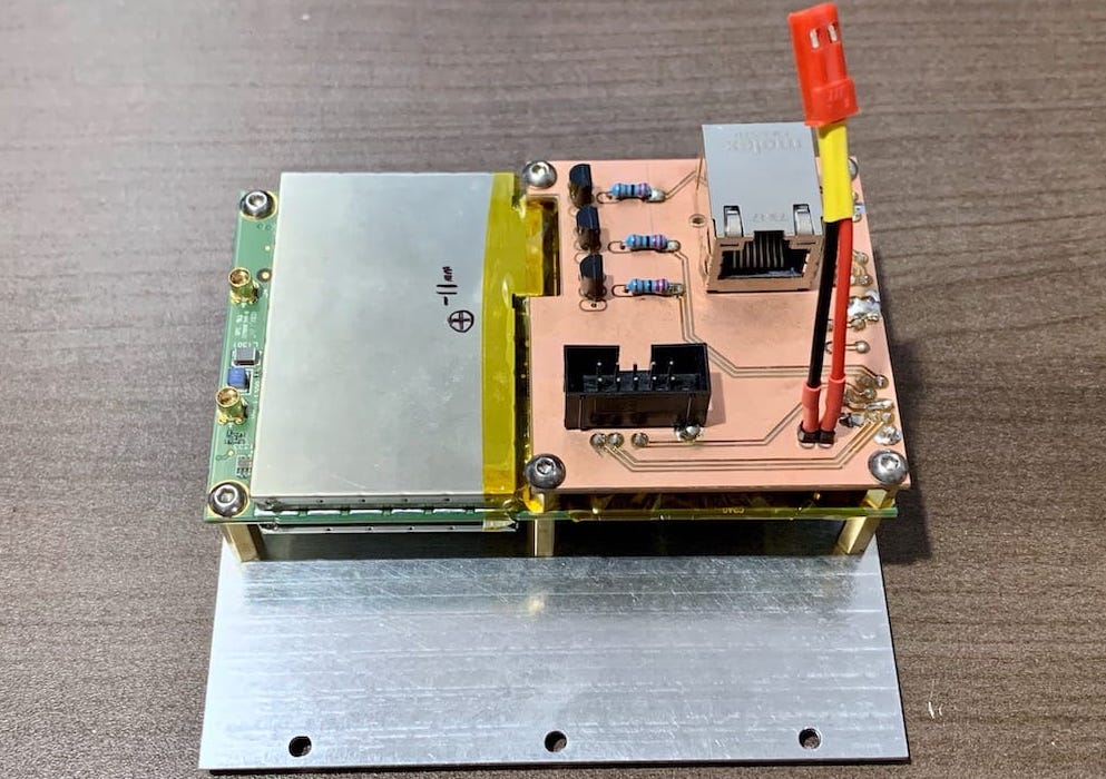
11.4. Left Face Assembly
The following components are needed to assemble the left face of the OpenMMS case.
2 @ 3mm (M3) button-head bolts, 8mm in length with flat washers and Nyloc nuts
4 @ 3mm (M3) button-head bolts, 10mm in length with Nyloc nuts
22 AWG 2-pin JST power connector, 2cm in length
26 AWG 2-pin Futaba/JR connector, 2cm in length
10-wire ribbon cable with a connector on one end, separated wires on the other end, 8cm in length (built previously)
Ethernet cable (Cat5/6) with RJ-45 connector on one end, twisted pairs on the other end, 10cm in length (built previously)
Heat-shrink tubing
2-pin Lemo 0B female connector with locking nut
Ethernet jack (Assmann A-2004-2-4-R)
2 @ 16mm SPDT latching pushbuttons with LED and locking nut (recommended one with a red LED and one with a green LED)
OpenMMS GNSS Brackets ID: 1 and 2
OpenMMS left face
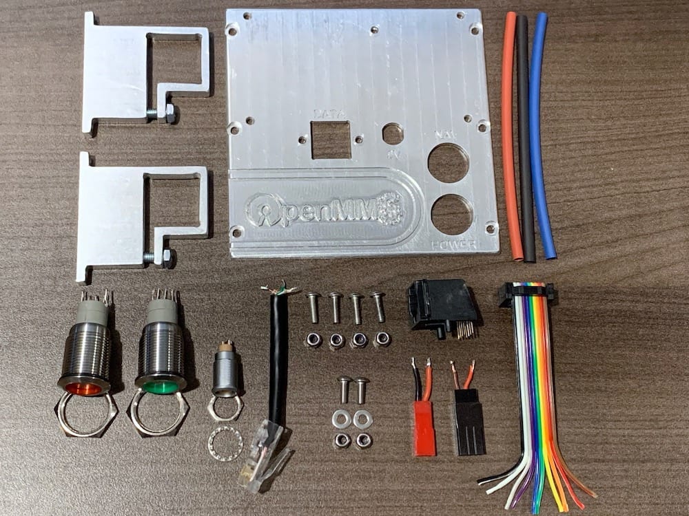
Fig 11.4-1. Components needed to assemble the left face
Start by snipping four of the eight wire connectors on the ethernet jack, see Figure 11.4-2 for specific details. Next, from the inside of the left face, insert the ethernet jack through the Data opening, ensuring the wire connectors are point up towards the top edge. Next, insert the two 8mm long M3 bolts into the holes on each side of the Data opening from the outside. Place flat washers followed by Nyloc nuts onto the 8mm long M3 bolts on the inside. Be sure the flat washers are sitting on an angle and covering the plastic tabs on the sides of the ethernet jack. Carefully tighten the bolts and Nyloc nuts until the ethernet jack is secure. Next, insert the 2-pin Lemo connector (with the red reference mark being at the top) along with the two 16mm latching pushbuttons into the left face, from the outside, and secure them using the respective locking nuts. It is recommended that the red pushbutton be on the bottom (i.e., will be the Power button) and the green pushbutton be on the top (i.e., will be the Navigation button).
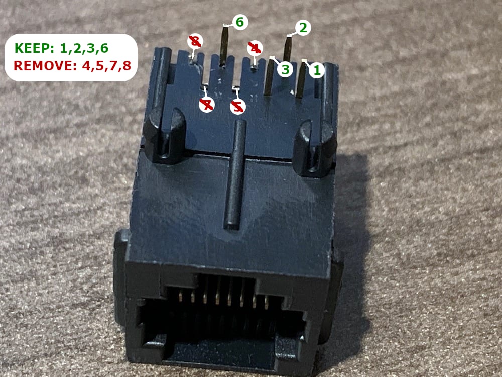
Fig 11.4-2. Ethernet jack wire connectors
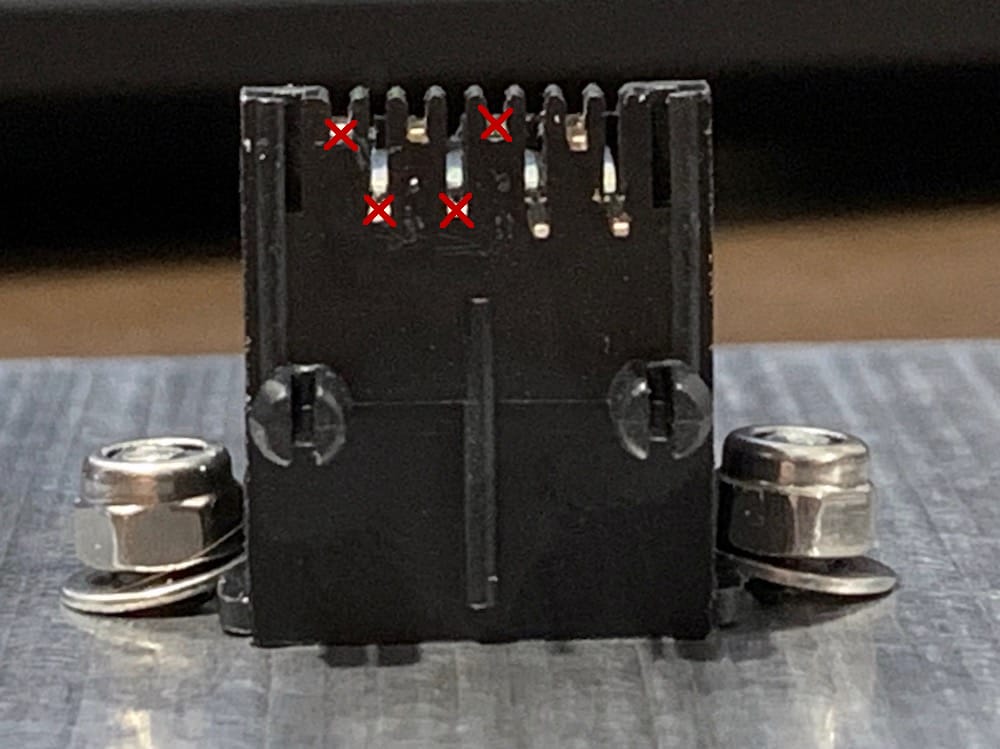
Fig 11.4-3. Ethernet jack installed
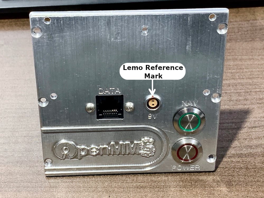
Fig 11.4-4. Lemo connector and pushbuttons installed
Next, solder the two twisted differential pairs of wires to the #1, #2, #3, and #6 wire connectors on the ethernet jack. Refer to Figure 11.4-5 for an example of the wire colors for the differential pairs. Depending on the ethernet cable being used, the wire colors may be different than shown. If in doubt, use a digital multimeter to check the continuity of the individual wire ends to the ethernet plug connectors at #1, #2, #3, and #6. Next, solder the 26 AWG 2-pin Futaba/JR connector to the back of the Lemo connector. The power (e.g., middle red) wire needs to be solder to the pin on the Lemo connector that corresponds to the reference mark on the front side of the Lemo connector. The ground wire (e.g., bottom brown) needs to be solder to the remaining pin on the Lemo connector. Before soldering the wires in place, insert the wires through small pieces of heat-shrink tubing. After soldering, use a heat gun to shrink the tubing around the wires to insulate them. Next, solder the 22 AWG 2-pin JST connector to the bottom-middle and bottom-right connectors on the Power pushbutton. Technically it does not matter which wire is soldered to which connector. Use heat-shrink tubing to insulate the wires. The bottom-left connector on the Power pushbutton is not used and should be snipped off the back of the pushbutton.
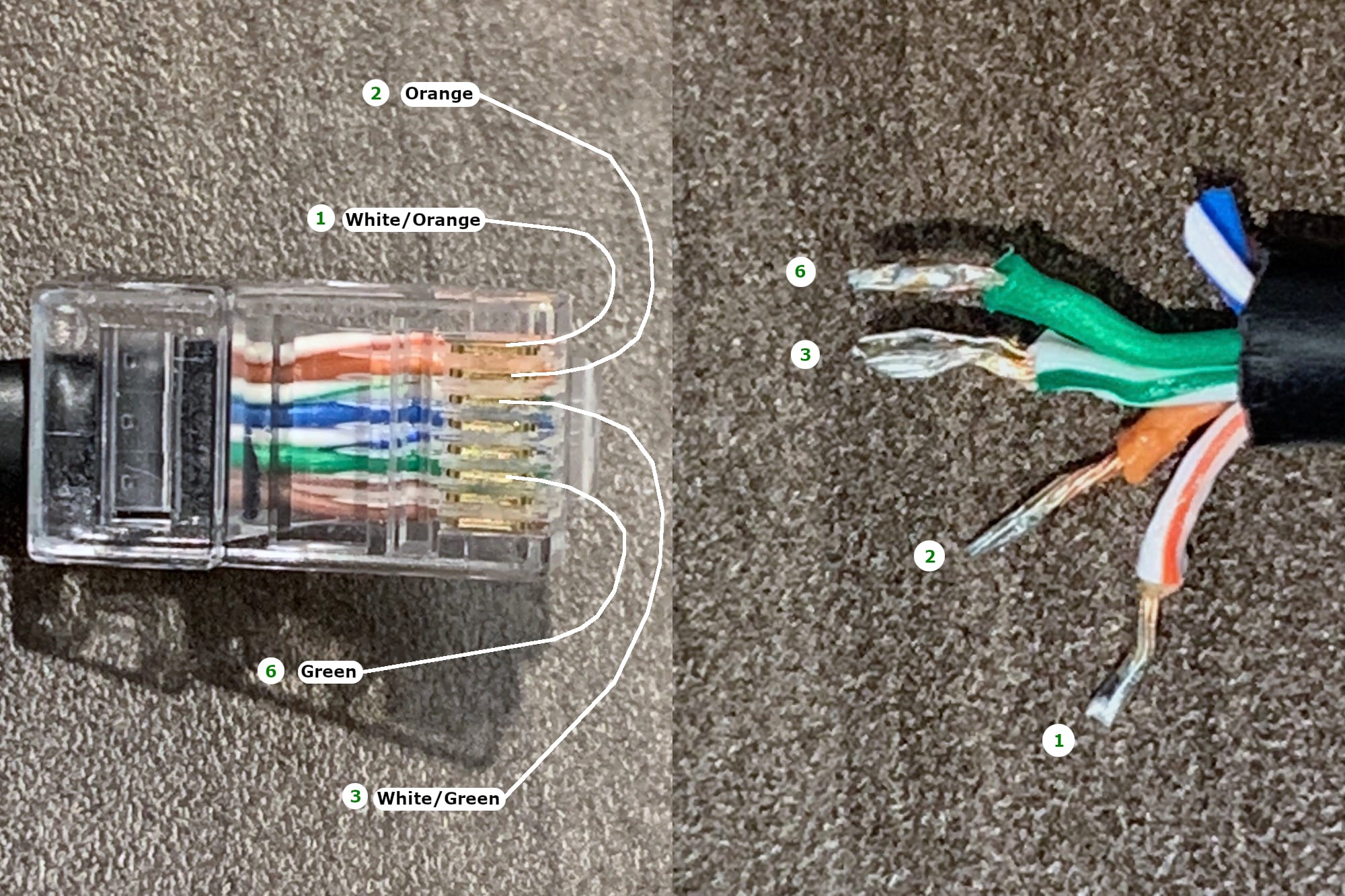
Fig 11.4-5. Ethernet cable wire colors
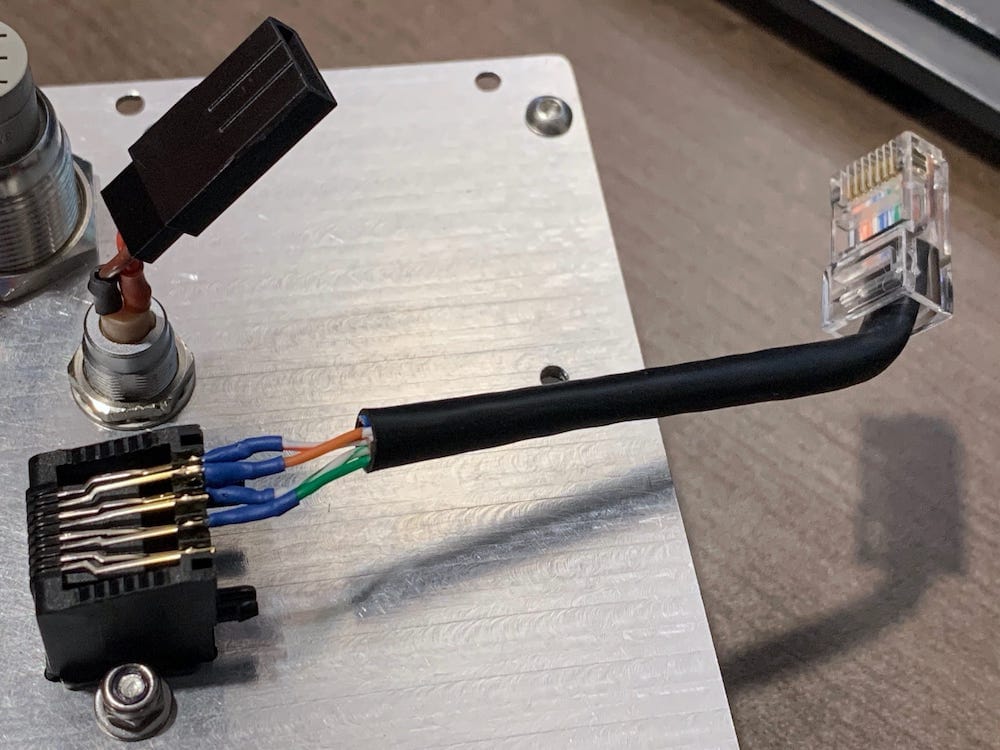
Fig 11.4-6. Ethernet cable and 9V power cable installed
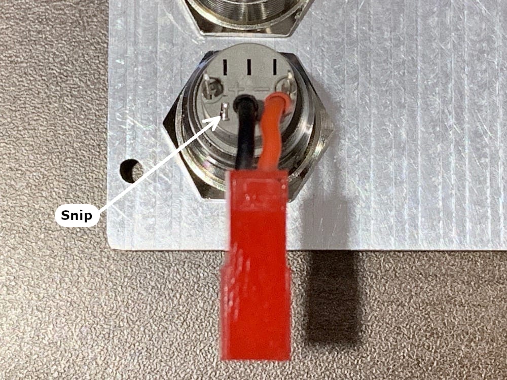
Fig 11.4-7. Unregulated system power cable installed
Next, refer to Figure 11.4-8 to understand which of the wires in the 10-wire ribbon cable need to be soldered to which connector on the Power pushbutton and Navigation pushbutton. Be cautious if the ribbon cable you are using has different color wires than those shown here. Next, insert two 10mm long M3 bolts from the inside of the left face through the front two holes for GNSS bracket 1. Thread the bolts into the drilled and tapped holes in the GNSS bracket until they are about to protrude from the other side of the bracket. Position a Nyloc nut tight against the other side of the GNSS bracket and continue threading the M3 bolt through the bracket and the Nyloc nut. You may or may not have room for the Nyloc nut to be rotated while tight against the bracket. Do your best to ensure that the Nyloc nuts are tight against the bracket. It may help to file the inside corner of the mounting tabs on the GNSS bracket to get a bit more room to install the Nyloc nut. Lastly, repeat this process for installing GNSS bracket 2 along the back edge of the left face.
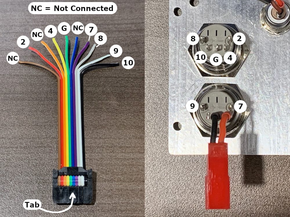
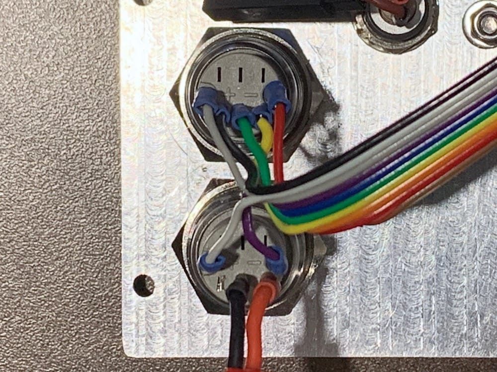
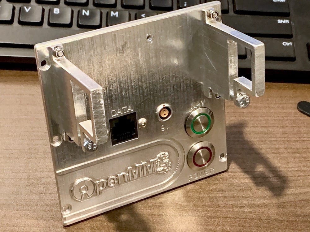
11.5. Right Face Assembly
The following components are needed to assemble the right face of the OpenMMS case.
4 @ 3mm (M3) button-head bolts, 5mm in length
4 @ 3mm (M3) button-head bolts, 10mm in length with Nyloc nuts
2 @ 3mm (M3) Female/Female standoffs, 6mm in length
2 @ 26 AWG 3-pin Futaba/JR connector, 2cm in length
Additional ~3cm length of 26 AWG wire
Heat-shrink tubing
4-pin Lemo 0B female connector with locking nut
16mm SPDT momentary pushbutton with LED and locking nut (recommended one with a blue LED)
Assembled OpenMMS LED Board V1.3
OpenMMS GNSS Brackets ID: 3 and 4
OpenMMS right face
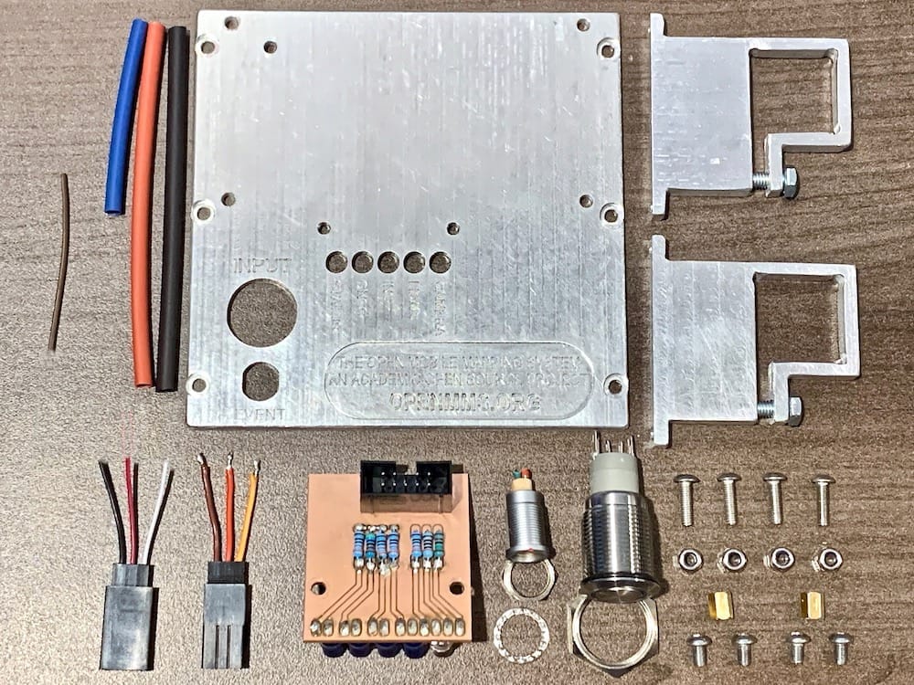
Fig 11.5-1. Components needed to assemble the right face
Start by inserting the 16mm SPDT momentary pushbutton into the Input hole, through the outside of the right face. Thread the locking nut onto the pushbutton on the inside of the case. The bottom-left connector on the Input pushbutton is not used and should be snipped off the back of the pushbutton. Next, insert the 4 pin Lemo connector into the Event hole, ensuring that the connectors’ reference mark faces the top edge of the face. Secure it in place on the inside of the face using the locking nut. Next, strip one end on the additional 3cm 26 AWG wire and twist it together with the ground wire (outside wire) on one of the Futaba/JR 3-pin connectors and then solder them together. Solder this 2-wire connection to the bottom-middle wire connector on the pushbutton, be sure to use heat-shrink tubing to insulate the wire. Next, strip the other end of the 3cm wire and solder it to the upper-right wire connector on the pushbutton. Next, the middle wire on the 3-pin Futaba/JR connector is soldered to the bottom-right wire connector on the pushbutton. Solder the remaining the Futaba/JR connector wire to the upper-left wire connector on the pushbutton.
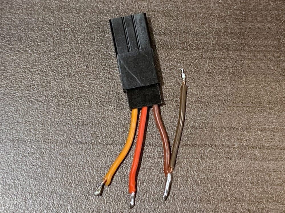
Fig 11.5-2. 2-wire ground connection
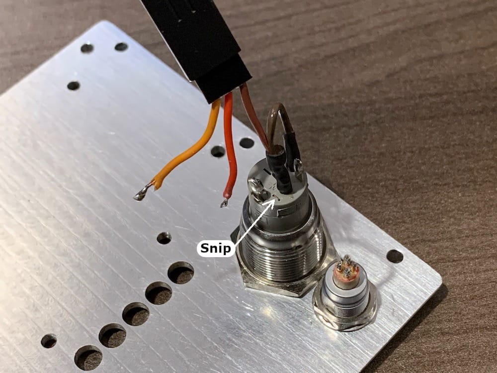
Fig 11.5-3. Ground wires soldering is complete
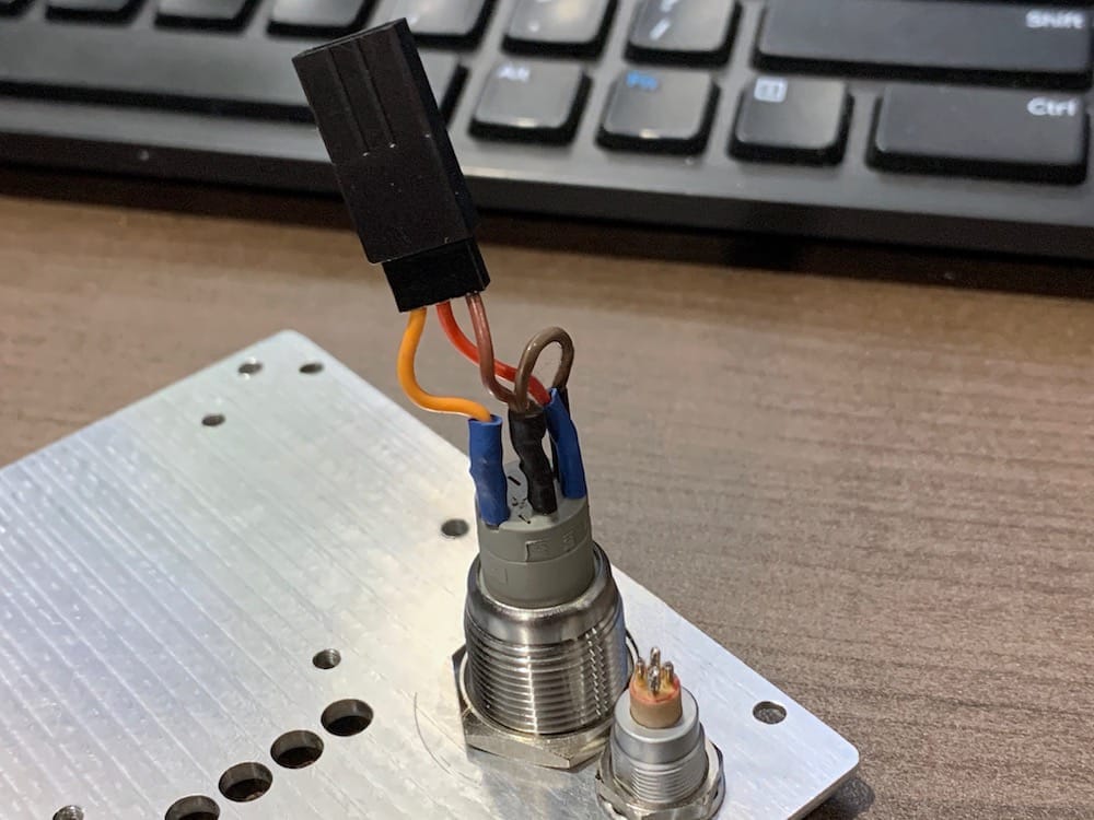
Fig 11.5-4. Input pushbutton completed
Next, solder the outside (white) wire of the 2nd Futaba/JR 3-pin connector to the upper-right wire connector on the Lemo connector. Solder the middle (red) wire of the 2nd Futaba/JR 3-pin connector to the upper-left wire connector on the Lemo connector. Lastly, solder the other outside (black) wire to BOTH bottom wire connector on the Lemo connector.
Next, from the outside of the right face insert two 5mm long M3 bolts into the holes just above the five LED holes. On the inside of the face, thread the two M3 Female/Female standoffs onto the bolts and tighten. Carefully install the assembled OpenMMS LED Board V1.3 on the right face using two 5mm long bolts, see the previous instructions provided in the LED Board assembly section for further details. Lastly, install GNSS brackets 3 and 4 onto the right face, see the Left Face Assembly section for the specific instructions on how to install a GNSS bracket.
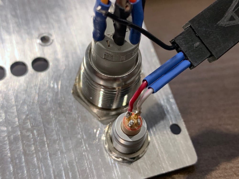
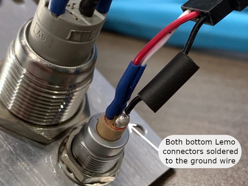
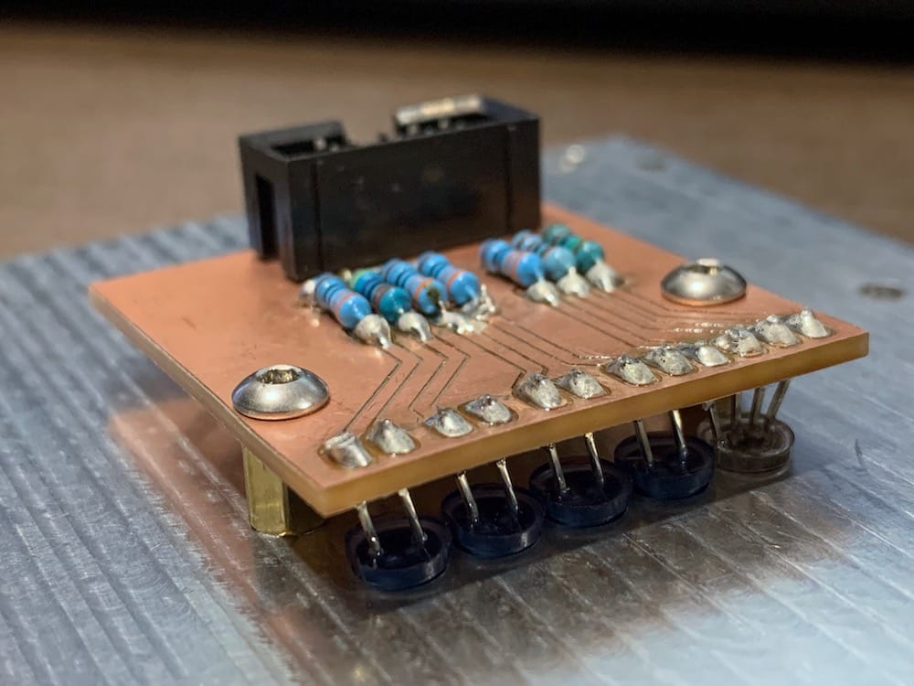
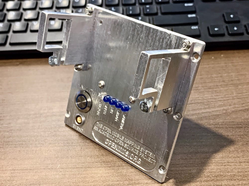
11.6. Front Face VLP-16 Installation
The following components are needed to install a Velodyne VLP-16 lidar sensor on the front face of the OpenMMS case.
2 @ 4mm (M4) hex bolts, 10mm in length with lock washers
1 @ 1/4” coarse thread hex bolt, 1/2” in length
4 @ 3mm (M3) Male/Female standoffs, 12mm in length
Velodyne VLP-16 Puck (or Puck-Lite) lidar sensor with its cable cut to 25cm in length, with 2cm of exposed wires at the cable’s end, with ~3mm stripped wire ends
OpenMMS front face (VLP-16)
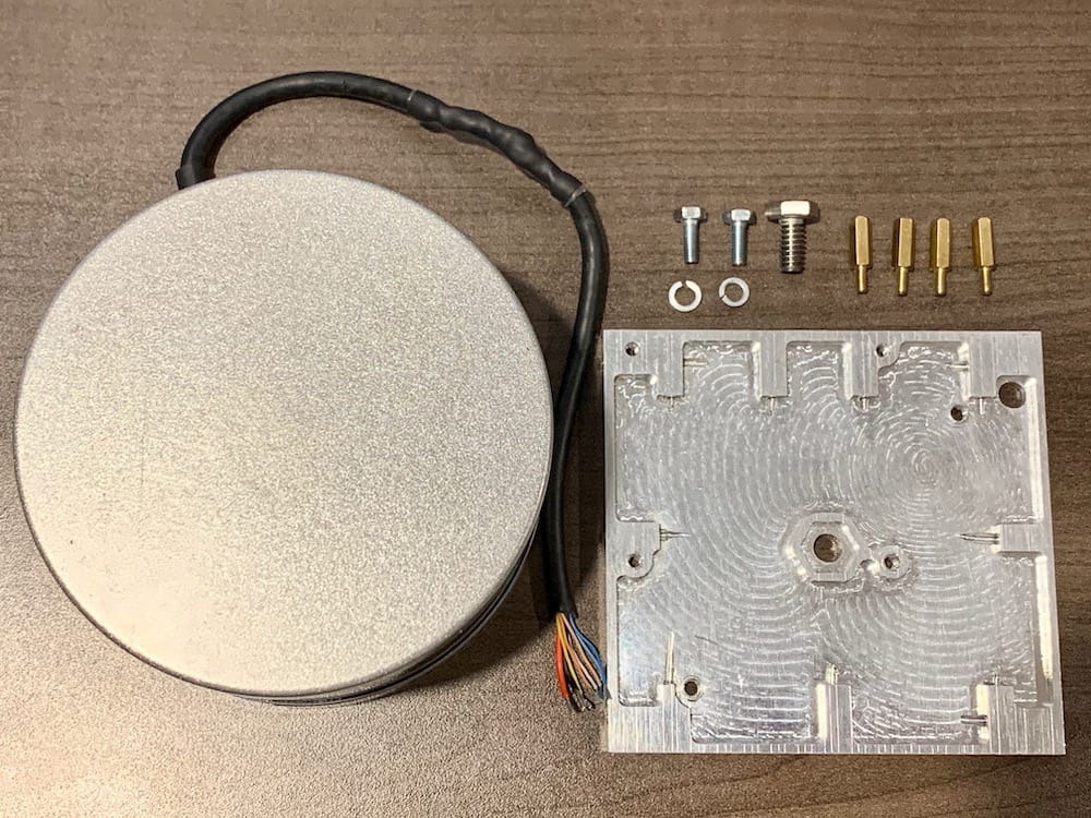
Fig 11.6-1. Components needed to install a Velodyne VLP-16 lidar sensor
Start by making a mark on one of the corners of the 1/4” hex bolt and positioning it within the center hole of the front face. Notice that the front face has an aluminum ‘lock’ around the center hole that stops the bolt from rotating. Make reference to where the mark on the bolt is positioned with respect to the aluminum lock. Hold the bolt in place and thread the center hole in the bottom of the VLP-16 sensor onto the bolt and rotate the front face until it is tight against VLP-16. If lucky, the cable of the VLP-16 will be nearly aligned with the bottom-right corner of the face. Most likely, however, the cable will not be near the bottom-right corner. Examine the mark made on the bolt and use it to estimate where the bolt needs to be positioned within the aluminum lock to have the VLP-16 cable near the bottom-right corner. Next, loosen the front face until the bolt is free from the aluminum lock and re-position it as estimated. Re-tighten the front face and check if the cable is in the proper location. The VLP-16 needs to be snug against the front face but it does not need to be extremely tight. The final position of the VLP-16 will be achieved when the two threaded holes in the upper-right and lower-left corners of the front face visually align with the corresponding holes in the bottom of the VLP-16. Once aligned, the M4 hex bolts with lock washers can be threaded through these two holes and tightened.
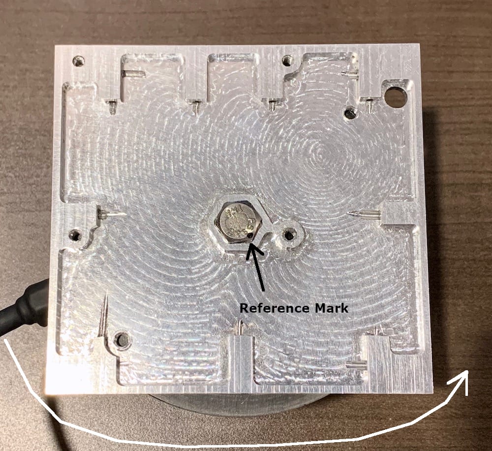
Fig 11.6-2. Wrong bolt location
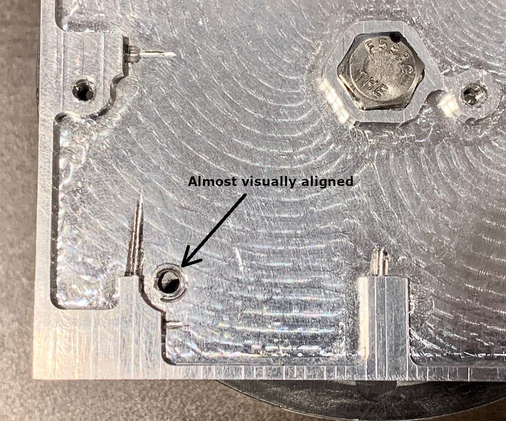
Fig 11.6-3. Almost at the final position
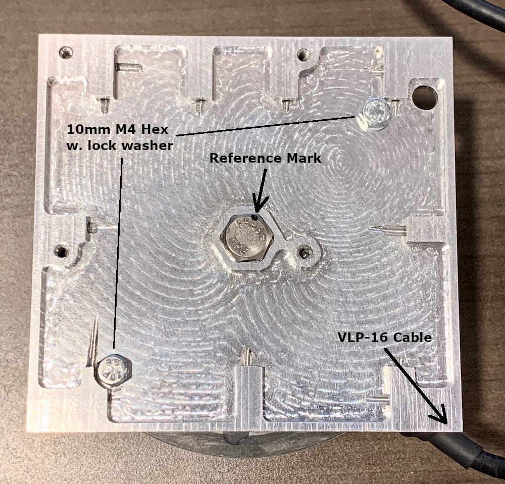
Fig 11.6-4. VLP-16 installed
Next, thread the four M3 Male/Female standoffs into the holes on the inside of the front face. BE CAREFUL WHEN TIGHTENED THE STANDOFFS AS M3 BRASS OR ALUMINUM STANDOFFS CAN BREAK WITHOUT APPLYING MUCH FORCE! Lastly, pass the VLP-16 cable through the hole in the upper-right corner of the face. The cable should be loose within hole. Mark the cable a little ways past the hole (i.e., the cable on the inside of the face). Cut a small length of heat-shrink tubing and slide it over the cable and align it with the mark. Use a heat gun to affix the heat-shrink tubing onto the cable. Depending on the thickness of the heat-shrink tubing being used, several layers may be affixed on top of one another until the cable fits snugly within the hole in the front face. The purpose of the heat-shrink tubing it to protect the cable as it passes through the aluminum and to create a seal between the cable and the front face.
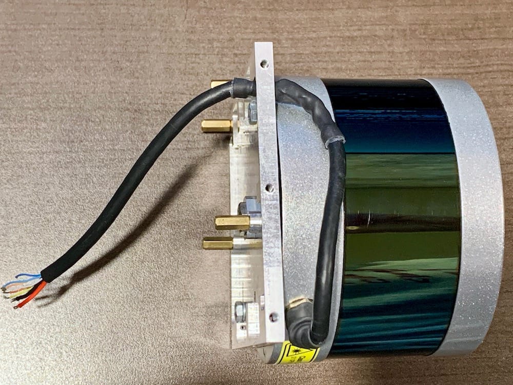
Fig 11.6-5. VLP-16 cable with heat-shrink tubing through the front face
11.7. Front Face MID-40 Installation
The following components are needed to install a Livox MID-40 lidar sensor on the front face of the OpenMMS case.
4 @ 3mm (M3) socket cap screw bolts, 10mm in length (taken from the bottom of the MID-40)
4 @ 3mm (M3) Male/Female standoffs, 12mm in length
Livox MID-40 lidar sensor with cable cut to 9cm in length, with 2cm of exposed wires at the cable’s end, with ~3mm stripped wire ends
OpenMMS front face (MID-40)
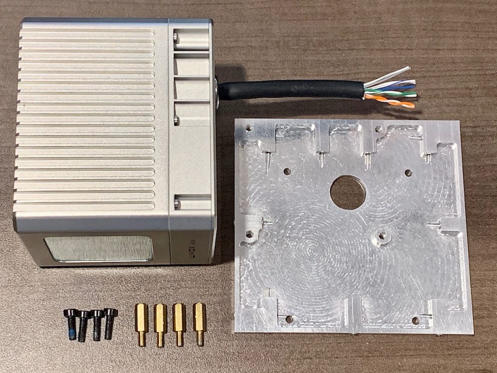
Fig 11.7-1. Components needed to install a Livox MID-40 lidar sensor
Start with removing the Livox Mounting Adapter from the bottom the MID-40 by removing the four M3 socket cap screw bolts using a 2.5mm Allen wrench/key. These four bolts will be reused to mount the MID-40 to the front face. Next, pass the MID-40 cable through the large hole in the front face and visually align the four smaller holes with the threaded holes in the bottom of the MID-40. Thread the four M3 socket cap screw bolts into these holes and tighten them. Lastly, thread the four M3 Male/Female standoffs into the holes on the inside of the front face. BE CAREFUL WHEN TIGHTENED THE STANDOFFS AS M3 BRASS OR ALUMINUM STANDOFFS CAN BREAK WITHOUT APPLYING MUCH FORCE!
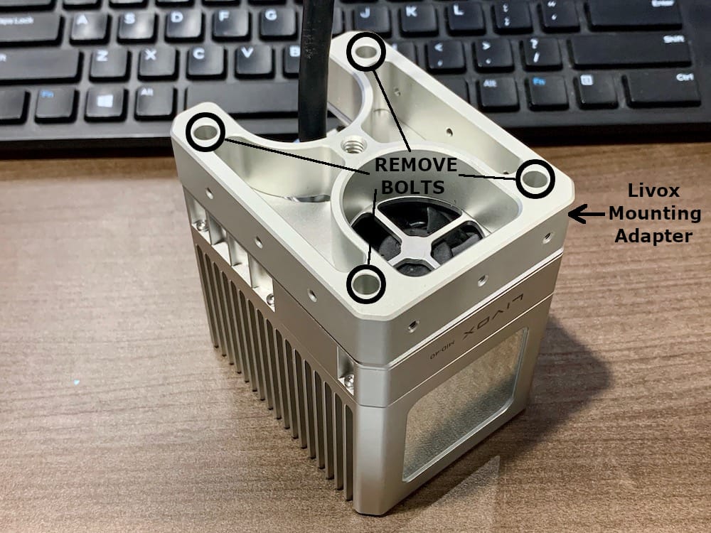
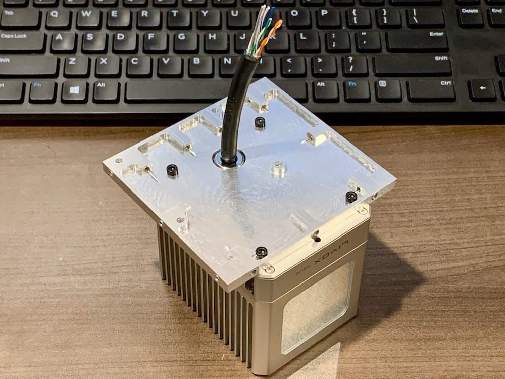
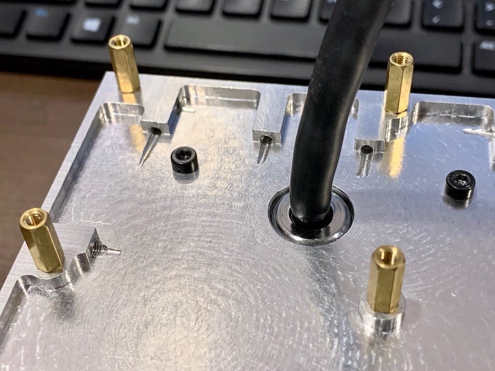
11.8. Front Face Assembly
The following components are needed to assemble the front face of the OpenMMS case.
4 @ 3mm (M3) button-head bolts, 5mm in length
3 @ 3mm (M3) Male/Female standoffs, 20mm in length
Raspberry Pi Camera ribbon cable, 15cm in length
Raspberry Pi 4 Model B computer
Assembled OpenMMS RPi Board V1.3
OpenMMS front face with an installed lidar sensor (VLP-16 or MID-40)
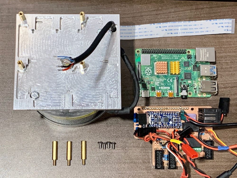
Fig 11.8-1. Components needed to assemble the front face (VLP-16 shown)
Start by manually threading an M3 bolt through each of the mounting holes in the Raspberry Pi computer. The mounting holes are designed for M2.5 bolts, but M3 bolts can be carefully threaded into the holes. Next, flatten the respective lidar cable against the inside surface of the front face. Position the Raspberry Pi computer over the standoffs (as shown in Figure 11.8-3) and thread a 5mm long M3 bolt through the bottom-left mounting hole and into the standoff. Thread a 20mm long M3 Male/Female standoff through the remaining three mounting holes on the Raspberry Pi and into their respective standoffs on the front face. Carefully tighten the bolt and the three standoffs, being sure not to apply too much force. Next, install the assembled OpenMMS RPi Board V1.3 onto the Raspberry Pi and secure it to the three 20mm long standoffs using the 5mm long M3 bolts.
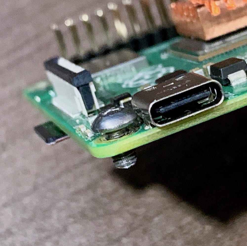
Fig 11.8-2. Thread M3 bolts in each hole
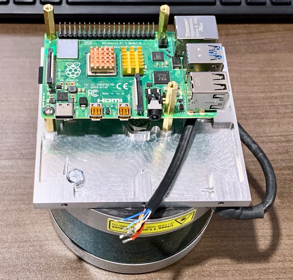
Fig 11.8-3. RPi 4 Model B installed
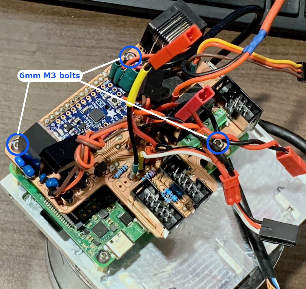
Fig 11.8-4. RPi Board V1.3 installed
Velodyne VLP-16 Wiring
Next, connect the lidar cable wires to the 8-wire terminal block on the RPi Board. Using a pair of tweezers can help to position the wires within the terminal block connectors. Ensure that the screws for each terminal block connector are tight enough to secure the wire, but do not overtighten them. The figure below shows how the wires for a Velodyne VLP-16 need to connect to the terminal block.
Livox MID-40 Wiring
Before the MID-40 sensor can be connected, a TTL to RS485 converter needs to be soldered to the RPi Board. Future versions of the RPi Board will include this signal conversion circuitry directly within the Board, but for the time-being this circuitry needs to be added as an external add-on.
The following components are needed to connect the TTL to RS485 external circuitry to the RPi Board.
MAX485 Circuit
3 x ~8cm lengths of 26 AWG wire
Heat-shrink tubing
2.2 Kohm resistor
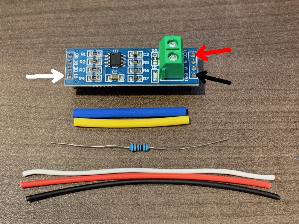
Fig 11.8-7. Components needed for TTL to RS485 external circuit
Start by removing the plastic collars around the pins on the bottom of the MAX485 circuit and then cutting/removing the pins EXCEPT for the the pins labelled DI, VCC, and GND (see figure below). Solder a red wire to the VCC pin, a black wire to the GND pin, and a white wire to the DI pin. Protect the soldered connections using heat shrink tubing. The red VCC wire needs to be soldered to one of the available 3.3V holes above the two 10-wire ribbon cable connectors on the RPi Board, and likewise the black GND wire needs to be soldered to one of the available GND holes on the RPi Board (see figure below). Next, position the thick MID-40 lidar cable under the Raspberry Pi and then secure it using a zip-tie to the standoff near the 8-wire screw terminal. Next, insert the white wire coming from the DI pin on the MAX485 circuit into the 3rd from the left screw terminal and tighten the connection. This connection is for the TTL pulse per second (PPS) signal coming from the APX-18 GNSS-INS sensor, which provides the precise time synchronization for the lidar observations.
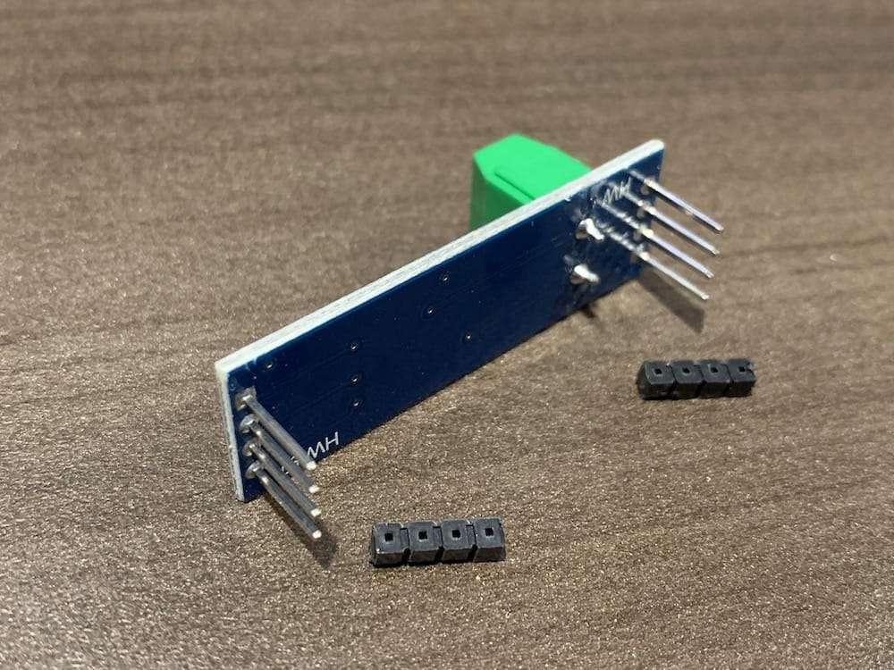
Fig 11.8-8. Plastic collars removed from bottom pins
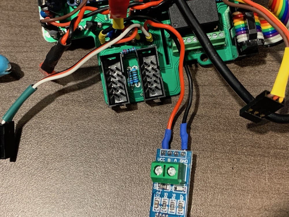
Fig 11.8-9. VCC and GND connected to the RPi Board
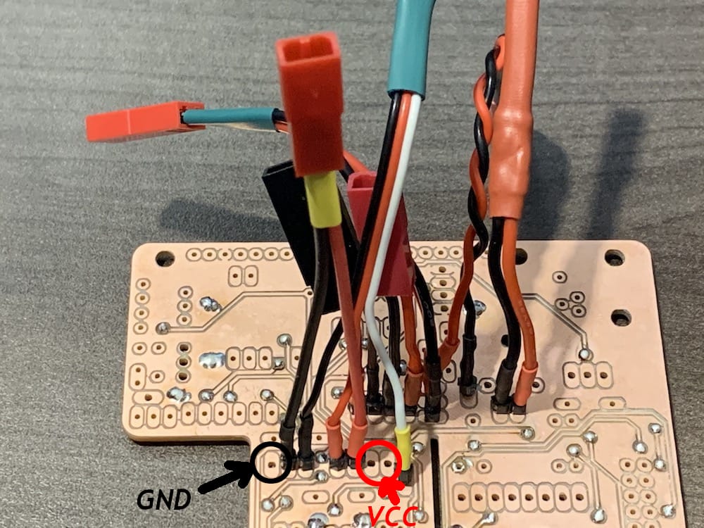
Fig 11.8-10. VCC and GND holes to use in RPi Board
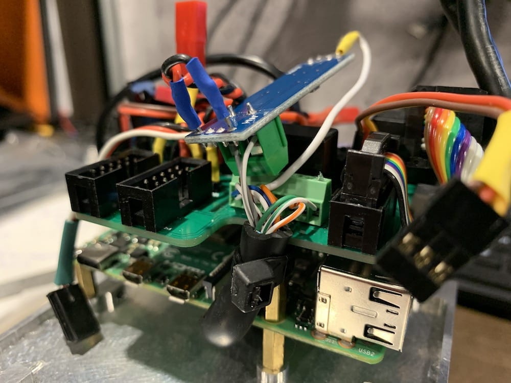
Fig 11.8-11. MID-40 lidar cable zip-tied in place
Next, the MID-40 lidar cable needs to be prepared before being connected to the RPi Board and MAX485 circuit screw terminals. See the figures below to understand what the purpose is for each of the colored wire within the lidar cable. The two POWER wires, colored BLUE and BLUE/WHITE need to be connected together. Likewise the two GROUND wires, colored BROWN and BROWN/WHITE need to be connected together. It is recommended to solder the tips of all eight of the wires within the lidar cable before connecting them to the screw terminals. Lastly, the 2.2 Kohm resistor needs to be carefully connected between the DI pin on the MAX485 circuit and 5th from the right pin on the RPi Board. The pin on the RPi Board corresponds to the header pins that connect to the Raspberry Pi computer. Be sure that the resistor’s bare wires do not come into contact with any other pins or soldered connections, it is recommended to encase the entire resistor within a piece of heat shrink tubing. The figure below shows an unprotected resistor only to help clarify the instructions. It is a tight fit, but the MAX485 external circuit does fit inbetween the RPi Board and the ethernet switch (when performing the final assembly of the OpenMMS case).
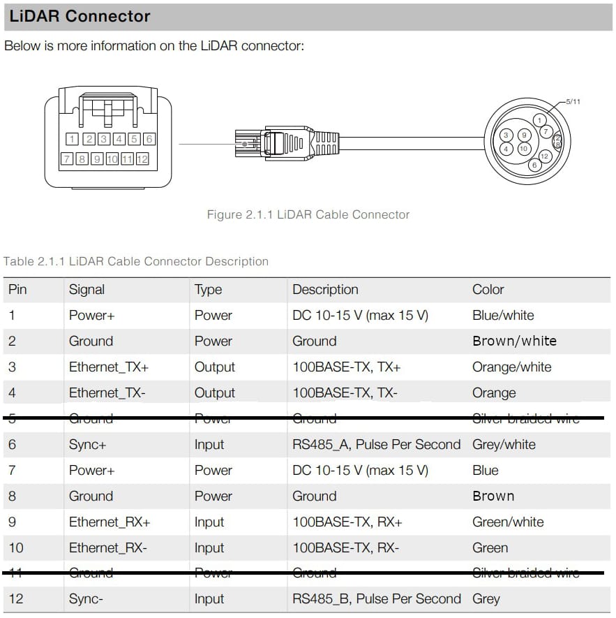
Fig 11.8-12. MID-40 lidar cable wiring information
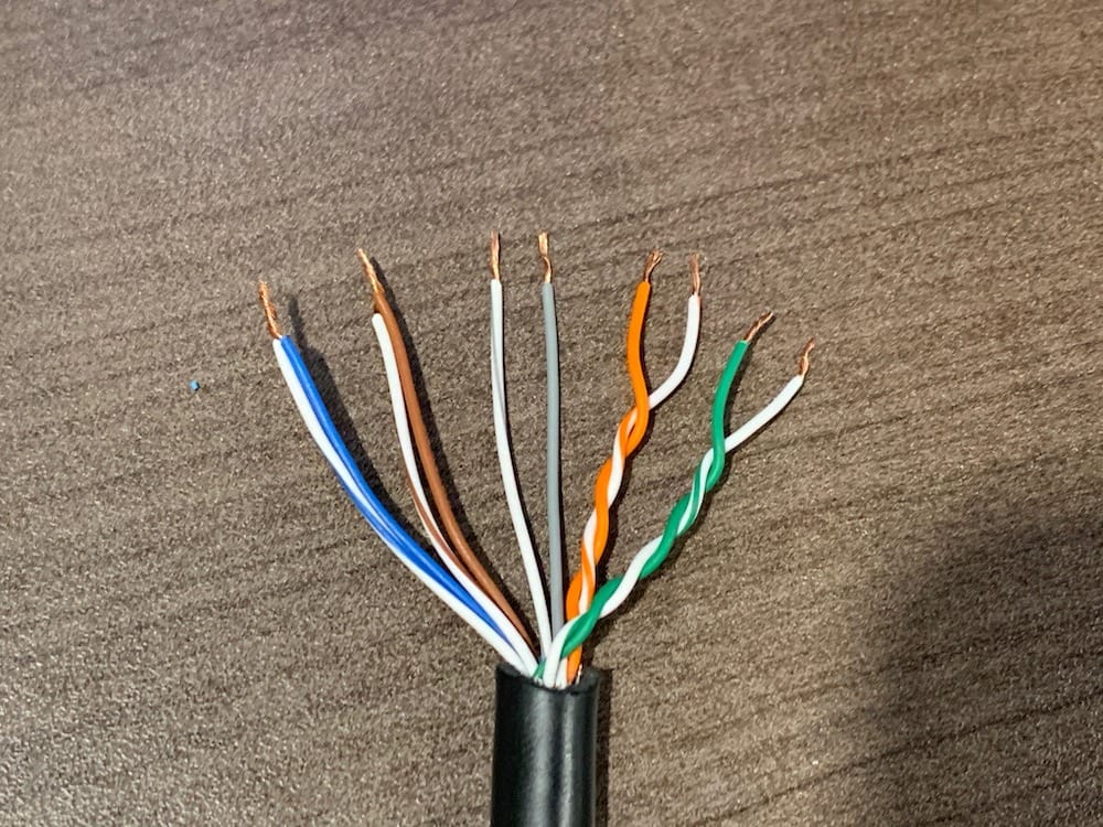
Fig 11.8-13. Prepared MID-40 lidar cable
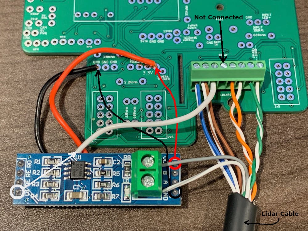
Fig 11.8-14. MID-40 lidar cable connections
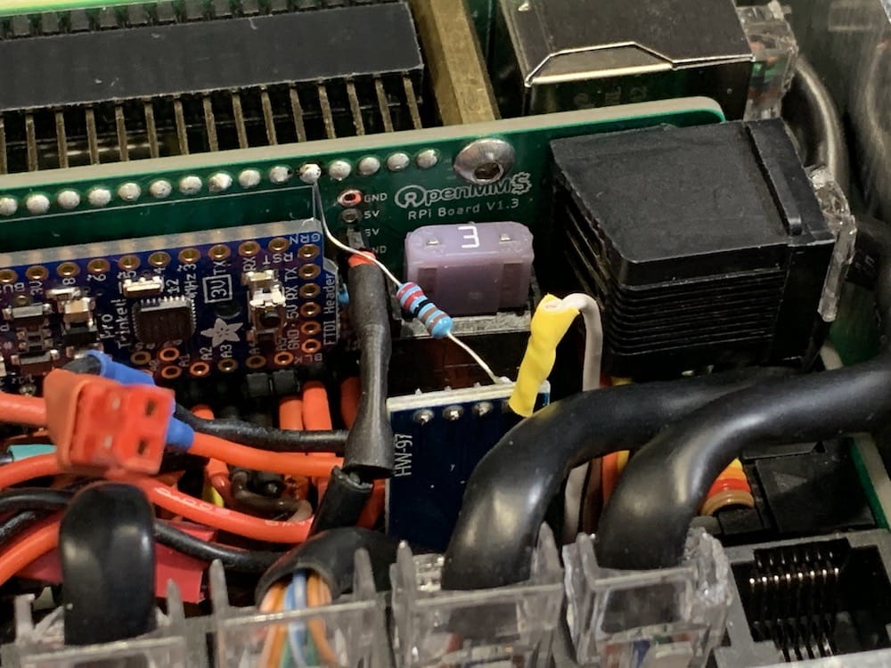
Fig 11.8-15. Resistor and MAX485 circuit installed
The final step in assembling the Front Face is to pass the Raspberry Pi Camera ribbon cable, with the blue side of the cable facing to the right, through the slot in the RPi Board. Ensure the camera connector on the Raspberry Pi computer is unlocked and insert the ribbon cable into it and then lock the connector.
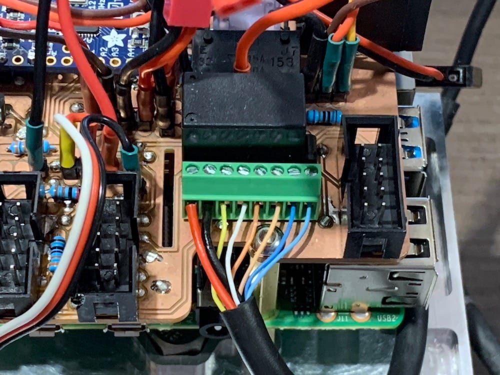
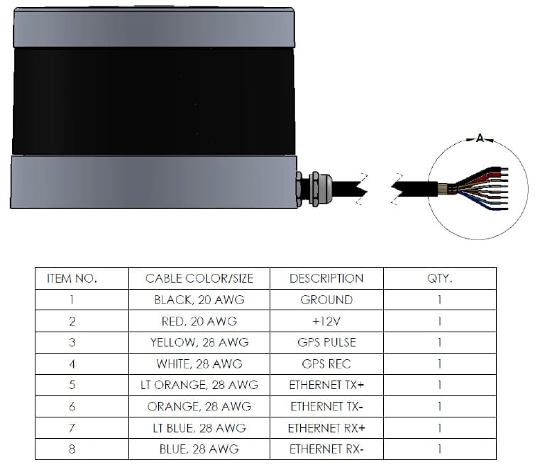
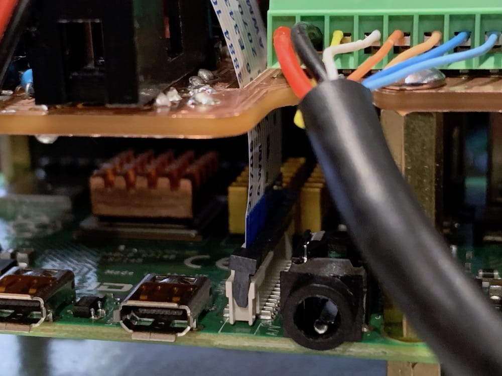
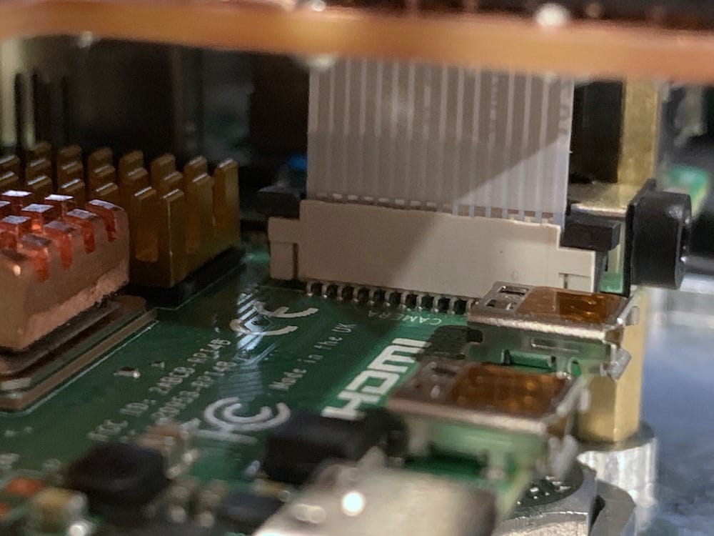
11.9. Back Face Assembly
The following components are needed to assemble the back face of the OpenMMS case.
2 @ 3mm (M3) button-head bolts, 5mm in length
2 @ 3mm (M3) button-head bolts, 8mm in length
1 @ 3mm (M3) button-head bolt, 14mm in length with a Nyloc nut
2 @ 3mm (M3) Female/Female standoffs, 10mm in length
2 @ 3mm (M3) Male/Female standoffs, 12mm in length
2 @ 4mm (M4) hex bolts, 10mm in length with lock washers
1 @ 1/4” coarse thread hex bolt, 1/2” in length with a lock washer
2 @ MMCX Female to SMA coaxial GNSS antenna cables
Strong double-sided foam tape
OpenMMS Support Board
Preconfigured Matek Systems UBEC Duo with shortened wires
Hak5 Micro ethernet switch
OpenMMS back face
OpenMMS Sony bracket
OpenMMS Sony trigger and event cable
Sony A6000 Camera
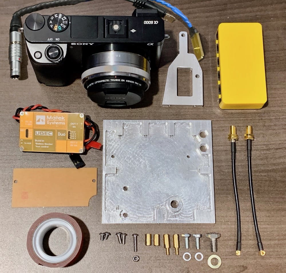
Fig 11.9-1. Components needed to assemble the back face
Start by inserting the 8mm M3 bolts through the two small holes in the outside of the back face. Then thread the two 10mm Female/Female standoffs to these bolts. Temporarily install the Support PCB to the standoffs, and mark the top and bottom edge of the Support PCB on the back face, then remove the Support PCB. Apply strips of strong double-sided foam tape to the front and back of the Matek Systems UBEC Duo power supply. Center the UBEC Duo between the marked lines and the standoffs on the back face and stick it in place. Ensure the wires are routed inside the standoffs and towards the top of the back face. Next, align the Support PCB with the standoffs and stick it to the front side of the UBEC Duo. Insert the 12mm M3 Male/Female standoffs through the holes in the Support PCB and tighten them (careful not to apply too much force).
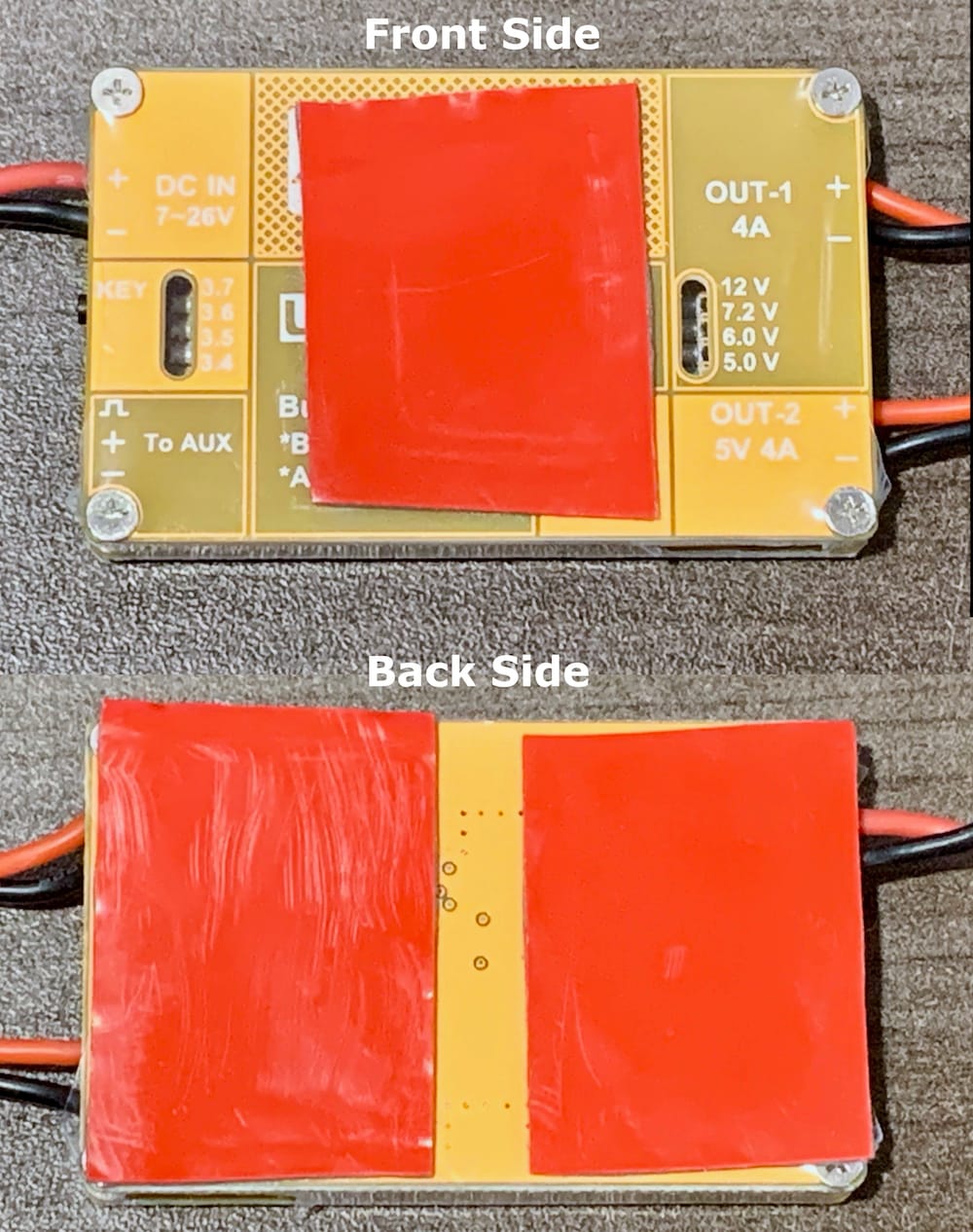
Fig 11.9-2. Double-sided foam tape on UBEC Duo
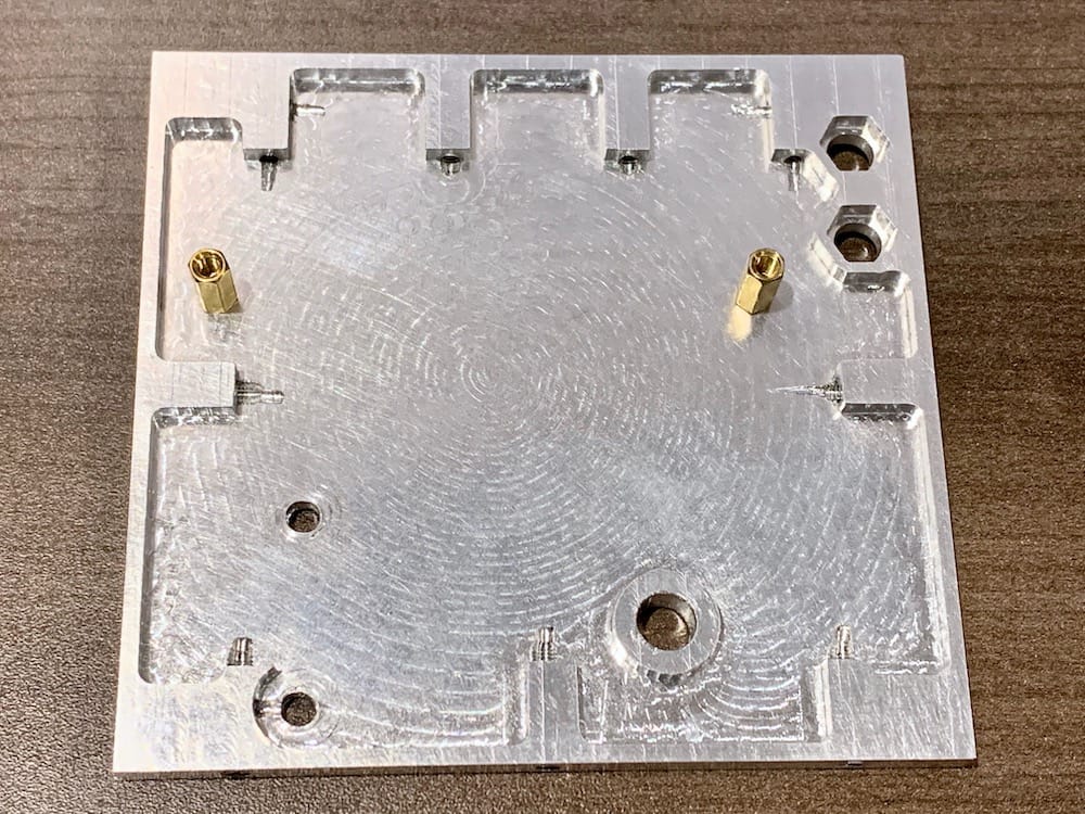
Fig 11.9-3. 10mm M3 standoffs
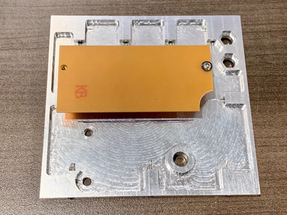
Fig 11.9-4. Support PCB temporarily installed
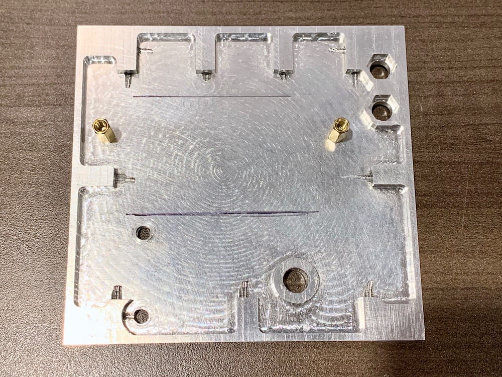
Fig 11.9-5. Support PCB top and bottom marks
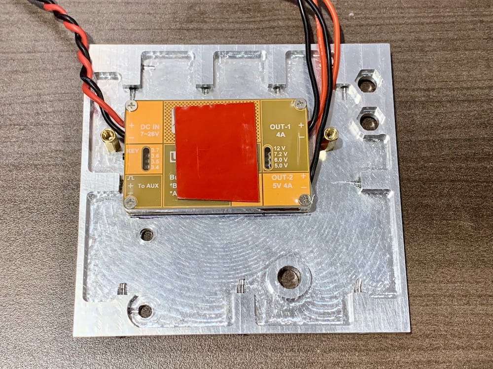
Fig 11.9-6. UBEC Duo positioned on back face
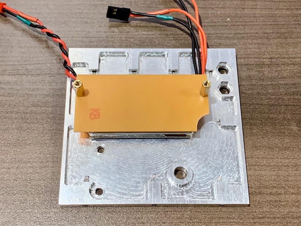
Fig 11.9-7. Support PCB installed
Next, the Hak Micro ethernet switch needs to be modified before it can be installed. Start by gently prying the plastic case apart using a small flat screwdriver. Starting at one of the case corners and separate the top and bottom parts of the case. Work around the edge of the case until the top and bottom pieces separate. Remove the ethernet switch from the case. Next, VERY CAREFULLY trim away the printed circuit board material from the outside edges of the ethernet switch near the small holes, which will create a notches on the edges of the board. Using a sharp X-Acto knife to scribe lines where the material will be cut helps avoid damaging the board. Notice that small electronic components are very close to these holes. Be sure not to damage these components. The notches need to be wide enough to have half of an M3 bolt fit within them. Next, on the back side of the ethernet switch, trim the excessively long wires of the through-hole components. Snip the wires as low as possible (being careful not to damage the soldered connections). Place double-sided foam tape over the backside of the ethernet switch to insulate the trimmed wires.
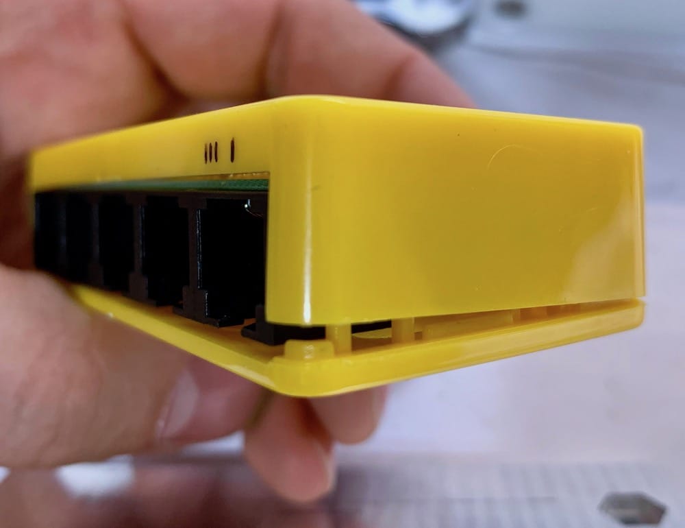
Fig 11.9-8. Prying the Hak5 case apart
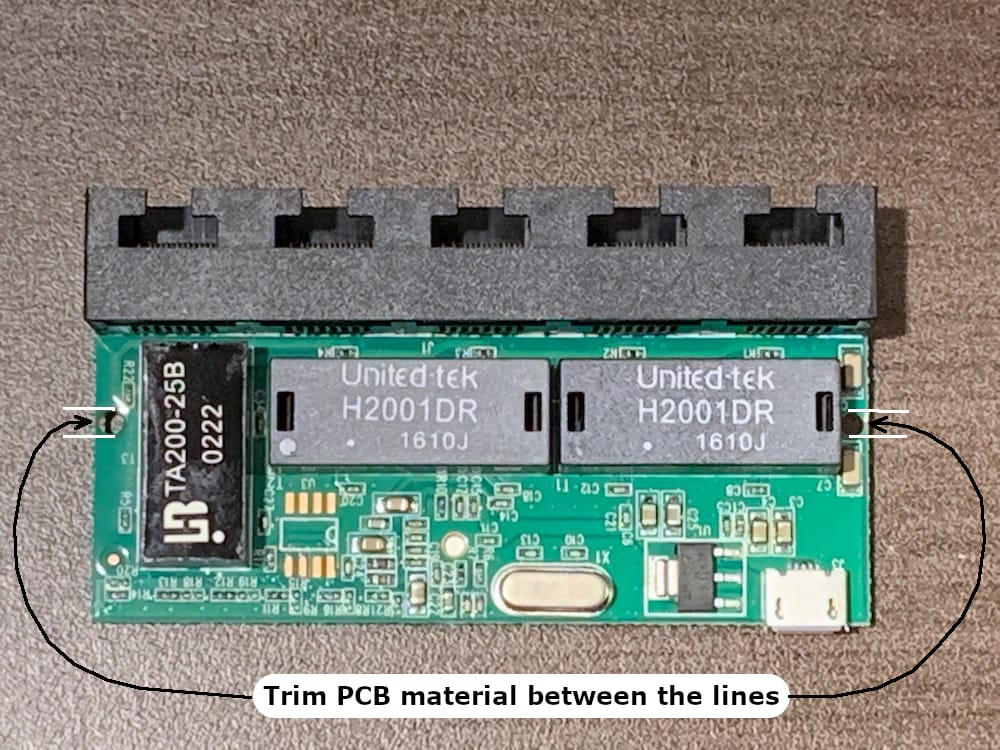
Fig 11.9-9. Ethernet switch with notch areas
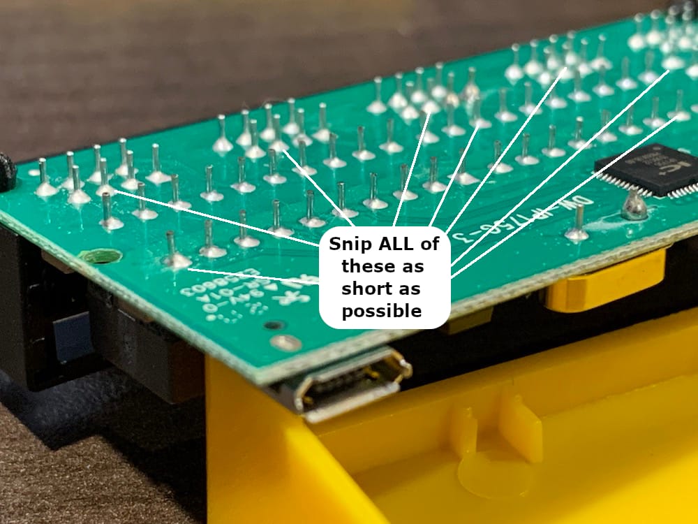
Fig 11.9-10. Long component wires to trim
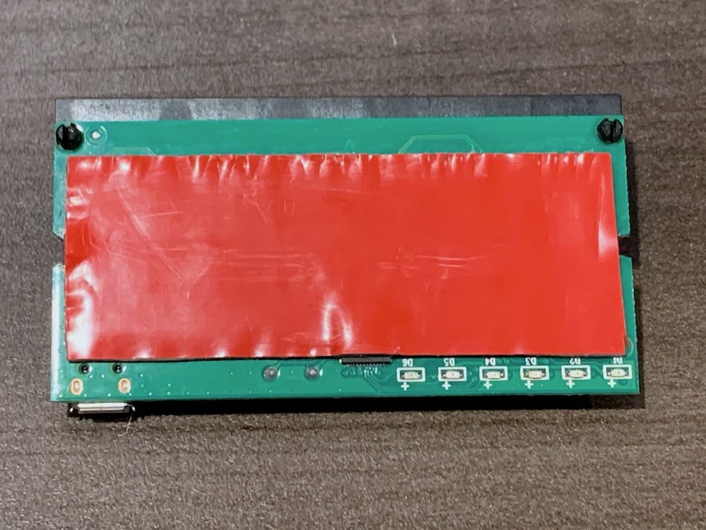
Fig 11.9-11. Insulate the Hak5 with foam tape
Next, add small pieces of double-sided foam tape to the top side of the ethernet switch over the notched areas. These pieces of tape are also used to provide insulation between the mounting bolts and the electrical components. Finally, the Hak5 Micro ethernet switch can be installed on the two 12mm standoffs on the back face. See Figure 11.9-13 to understand how the Hak5 must be oriented when being installed on the back face. Begin by threading a 5mm M3 bolt a couple of turns into one of the standoffs. Then slide the corresponding notched area of the Hak5 into the side of the bolt. Apply some sideways pressure to the ethernet switch pushing it into the bolt. Align the other notched area over the 2nd standoff and thread in the other 5mm M3 bolt. Once both bolts have been threaded, a couple turns into the standoffs, slowly begin tightening the bolts equally until they are moderately tight.
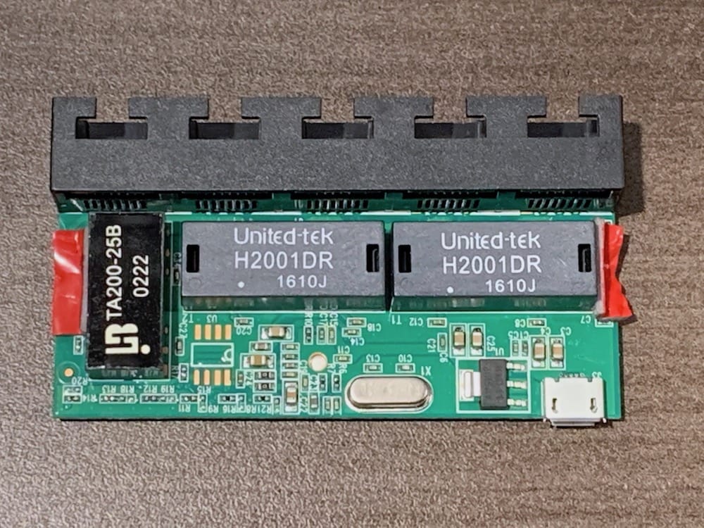
Fig 11.9-12. Tape for notch insulation
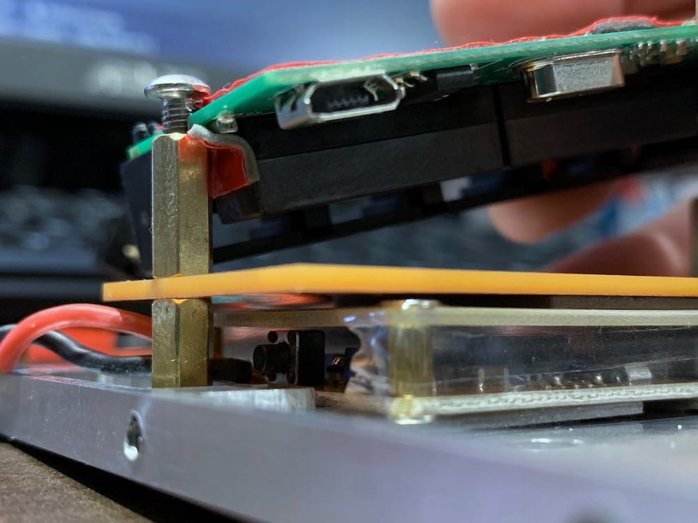
Fig 11.9-13. Slide one side against the bolt
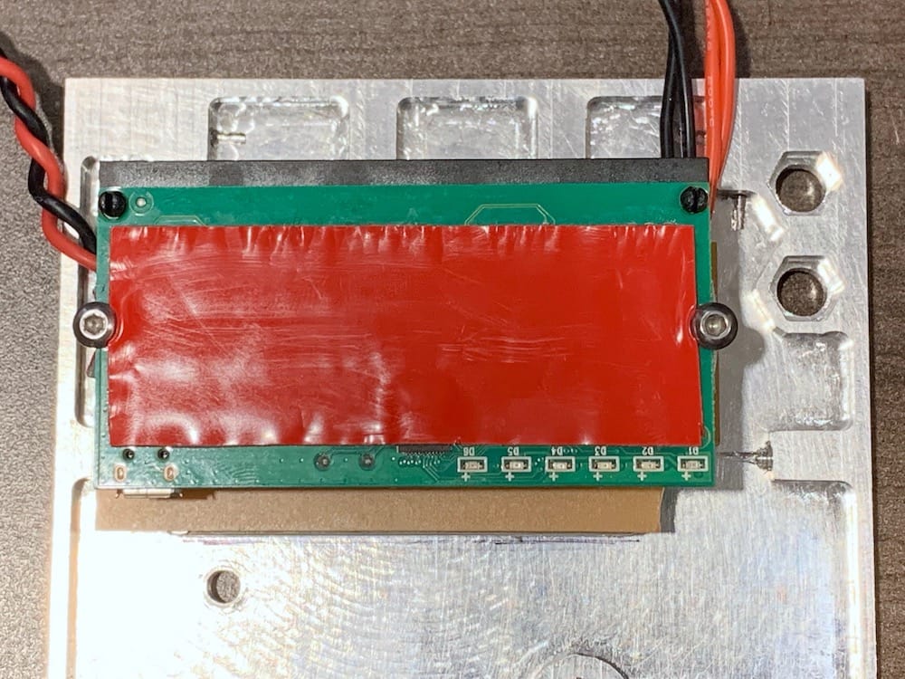
Fig 11.9-14. Hak5 Micro ethernet switch installed
Next, follow the instructions provided in the Aluminum Parts Manufacturing section, Drilling and Tapping Holes subsection, Sony Bracket Holes step, and install the Sony A6000 camera on the back face.
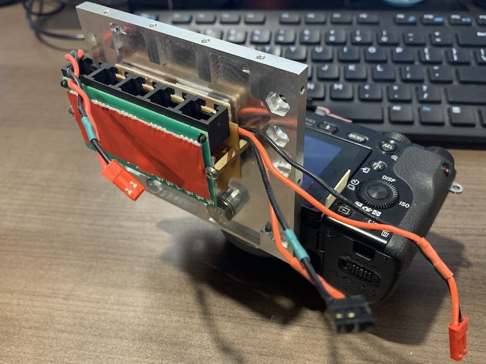
Fig 11.9-15. Sony A6000 camera installed
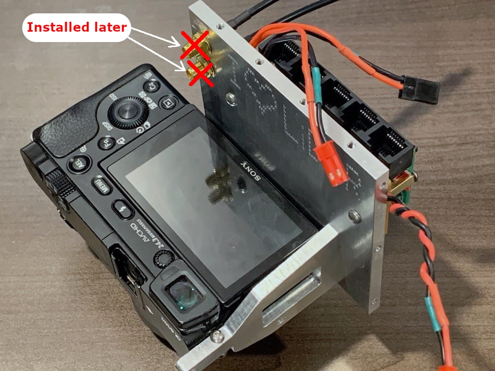
Fig 11.9-16. Assembled back face (minus trigger/event cable)
The OpenMMS Sony Trigger and Event cable is now installed. Begin by installing the TuffWing hot-shoe connector into the Sony A6000 camera. Ensure that the connector’s center metal pad correctly aligns with the reference line on the camera’s hot-shoe port. Use a hot-glue gun to apply a generous amount of glue around the TuffWing hot-shoe connector where it connects with the camera’s port. Allow the glue to cool naturally. It is recommended to apply a piece of high-strength double-sided foam tape over the hot-shoe (but do not remove the plastic film on the outside of the tape) . Next, flip the camera door open and insert the USB (multi) connector into the Multi port on the camera. This connection is used to trigger the shutter of the camera (i.e., take a photo). Next, loosely attach a zip-tie around the Event cable and through the upper hole in the Sony Bracket, and another loose zip-tie around the Trigger cable and the lower hole in the Sony Bracket. Gently pull down on the Trigger cable coming out of the camera and tighten the lower zip-tie when the cable is under a small amount of tension at the camera connector. Lastly, position the Event cable, so no tension occurs where the cable meets the PCB in the hot-shoe. Tighten the upper zip-tie to secure the position of the Event cable.
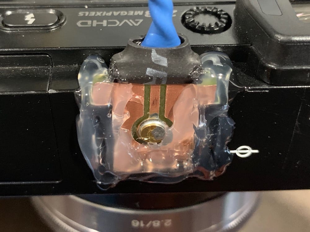
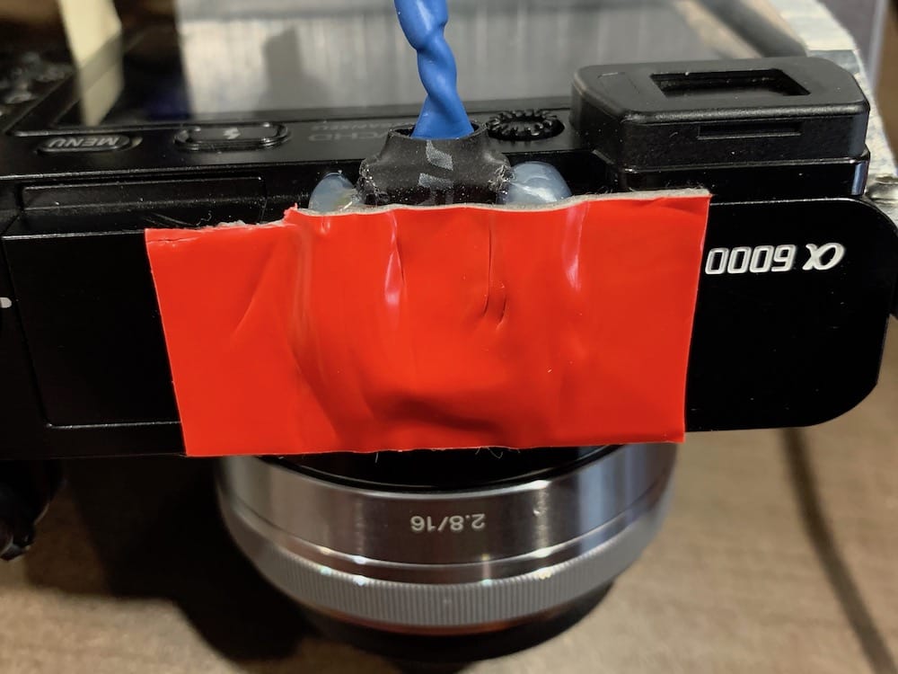
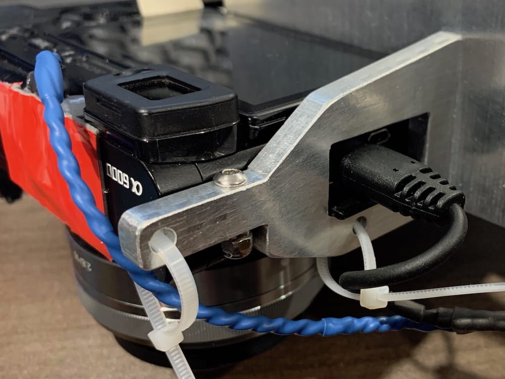
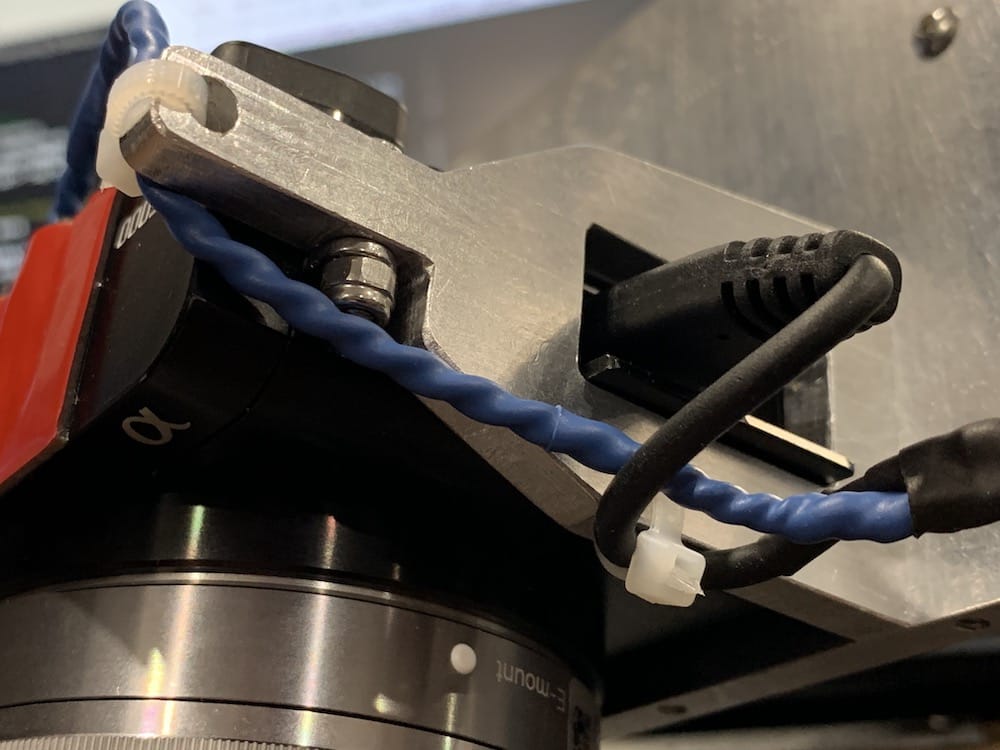
CONGRATULATIONS!
YOU HAVE NOW FINISHED ASSEMBLING ALL THE INDIVIDUAL ALUMINUM FACES OF THE OPENMMS CASE! THAT WAS ANOTHER BIG TASK!
12. Final Assembly
Important
When installing the final twenty-eight M3 bolts, it is strongly recommended that regular (medium strength), non-conductive Loctite be applied to the bolt. Within the instructions below, the use of Loctite is not mentioned only because of the instruction’s redundancy. It is also STRONGLY RECOMMENDED that the entire sensor be assembled at first, without the use of Loctite, to test the sensor’s operations (BUT NOT FOR TESTING FLIGHT OPERATIONS). Then, once the sensor is deemed operational, it should be taken apart and reassembled using Loctite on all bolts.
12.1. Overview
Alas, time for all the hard work to materialize into a physical and operational OpenMMS sensor! Due to the very tight placement of all the components inside the case, the order of operations for assembling the final sensor is very specific. Carefully and diligently read ALL of the following instructions before beginning the final assembly step.
The bolts required to assemble the OpenMMS sensor are:
8 @ 3mm (M3) button-head bolts, 14mm in length
18 @ 3mm (M3) button-head bolts, 12mm in length
2 @ 3mm (M3) button-head bolts, 8mm in length
12.2. Attach the Bottom Face
Begin by attaching the two ribbon cables and the two ethernet cables (one short and one long) into their respective connections on the Front Face Assembly. On the Bottom Face Assembly, attach the two MMCX to SMA coaxial cables to the APX-18 board and attach the remaining (long) ethernet cable to the ethernet jack on the OpenMMS APX-18 Board v1.3. Remove the star washer and locking nut from the ends of the coaxial cables. Install the Bottom Face Assembly on the Front Face Assembly using three M3 12mm long button-head bolts.
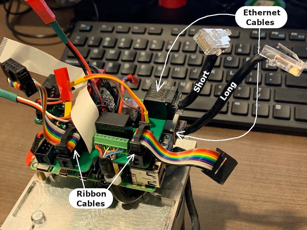
Fig 12.2-1. Front Face Assembly cables
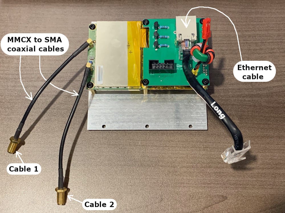
Fig 12.2-2. Bottom Face Assembly cables
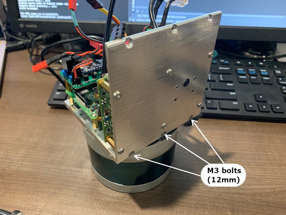
Fig 12.2-3. Bottom installed on Front
Next, connect the ribbon cable on the RPi Board to the APX-18 Board. Then connect the Raspberry Pi camera cable into the Raspberry Pi camera located underneath the APX-18 sensor. Be careful if any tools are used underneath the APX-18 when connecting the camera. Lastly, connect the yellow ID 2-wire JST 3.3V power cable from the RPi Board to the APX-18 Board. Installing these individual assemblies together creates what is now called, the Case Assembly.
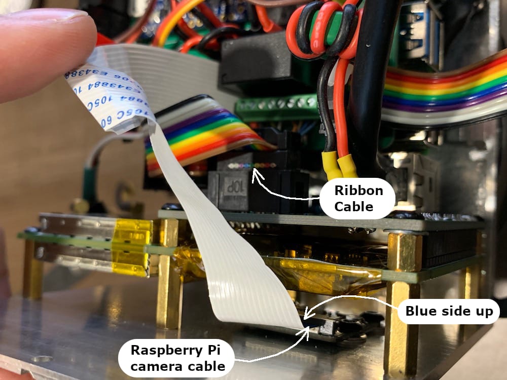
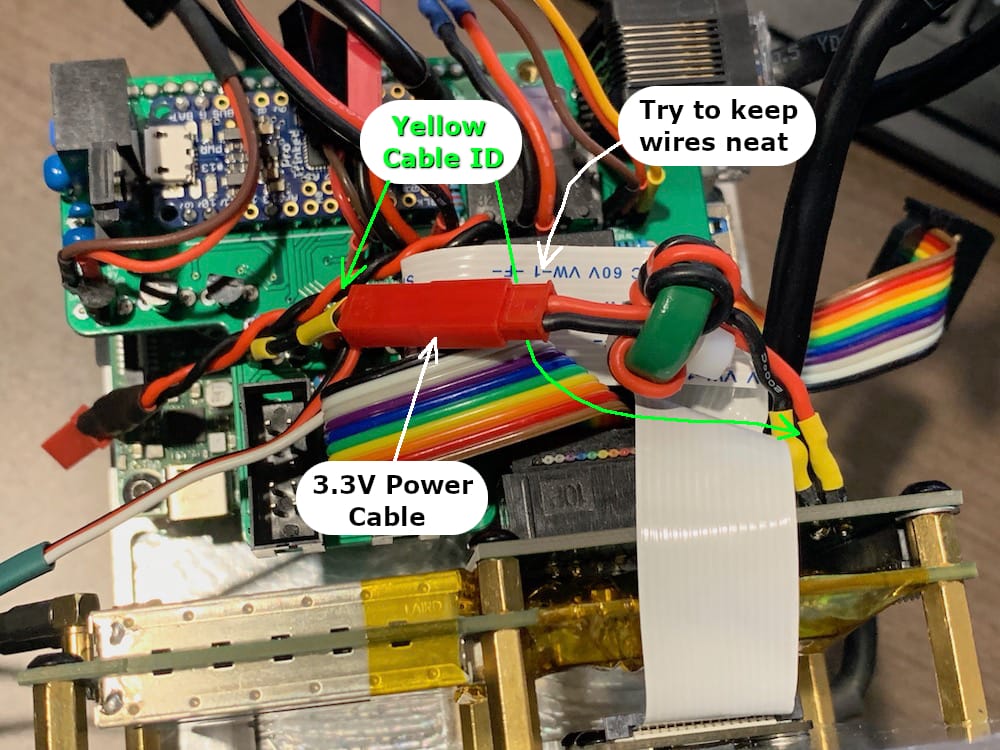
12.3. Attach the Side Faces
Begin by installing the Left Face Assembly onto the current Case Assembly. Connect the ribbon cable from the Left Face Assembly to the empty 2x5 connector on RPi Board. Be sure to support the back of the RPi Board when pushing the ribbon cable into the connector. Next, connect the Black ID JST cable to the POWER pushbutton, and then the Black ID 2-wire JR/Futaba cable to the 9V Lemo connector.
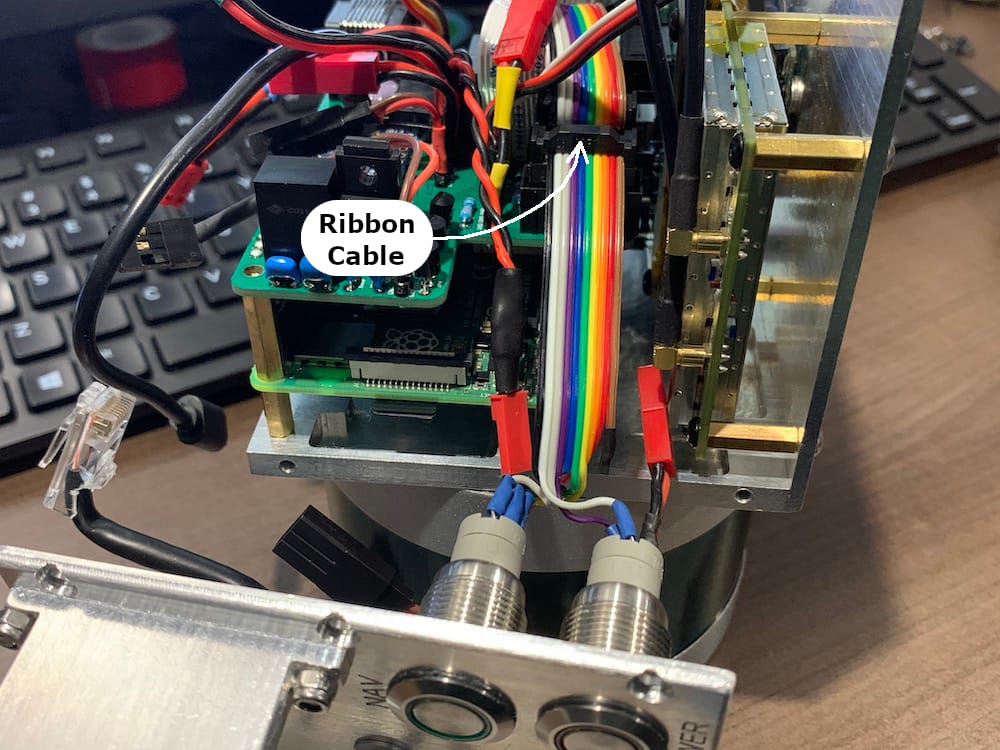
Fig 12.3-1. Left Face ribbon cable connected
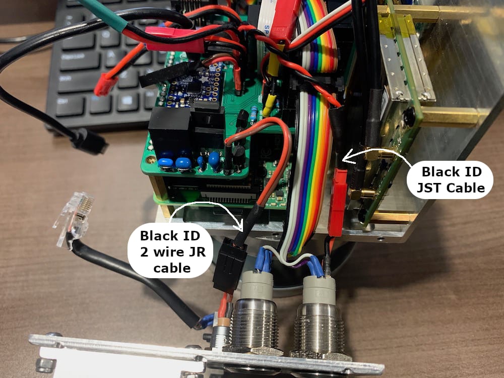
Fig 12.3-2. Black ID JST and JR/Futaba cables connected
Next, the two coaxial cables connected the APX-18 sensor need to be routed against the Left Face. The coaxial cable closest to the Front Face needs to be routed between the ethernet jack and the Lemo connector. The other coaxial cable needs to be routed between the Lemo connector and the pushbuttons. Lastly, slowly move the Left Face Assembly into position against the Case Assembly. Pay close attention that NO cables are pinched between the assemblies or other components. Align the three case holes between the Left Face Assembly and the Front Face Assembly and use three M3 12mm long bolts to attach them.
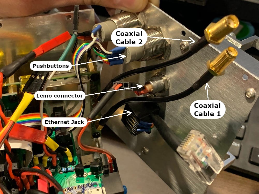
Fig 12.3-3. Coaxial cables routed around the Lemo connector
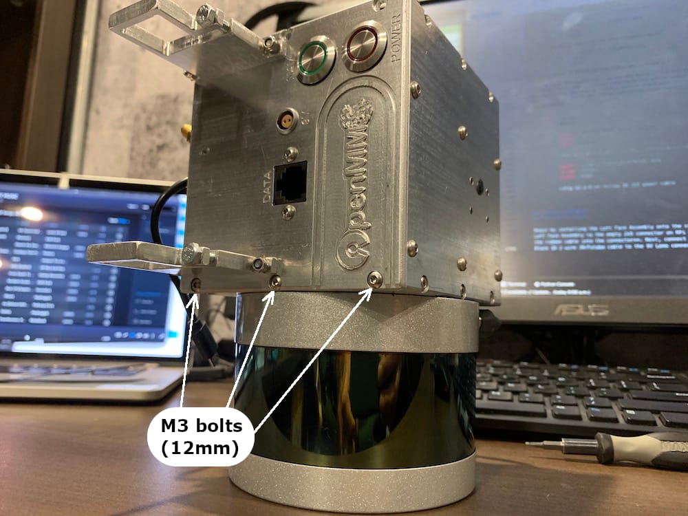
Fig 12.3-4. Left Face Assembly joins the Case Assembly
Continue by installing the Right Face Assembly onto the current Case Assembly. Connect the remaining ribbon cable from the RPi Board to the LED Board. Next, connect the Yellow ID and Green ID 3-wire JR/Futaba cables to the Input pushbutton and Event Lemo connector, respectively.
Finally, slowly move the Right Face Assembly into position against the Case Assembly. Pay close attention that NO cables are pinched between the Assemblies or other components. Align the three case holes between the Right Face Assembly and the Front Face Assembly and use three M3 12mm long bolts to attach them.
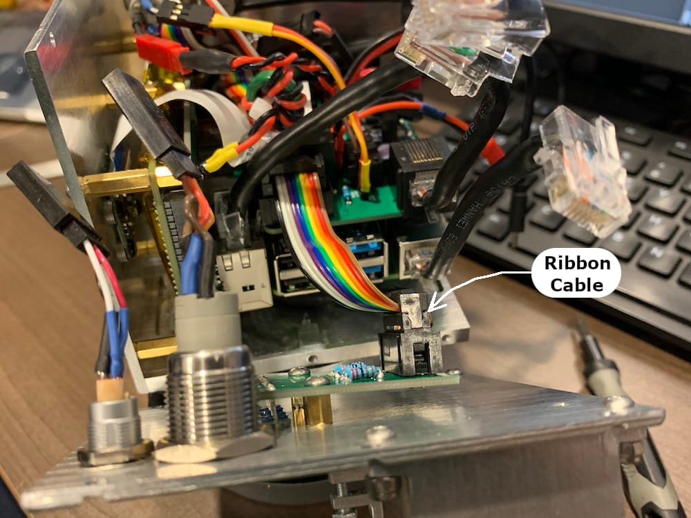
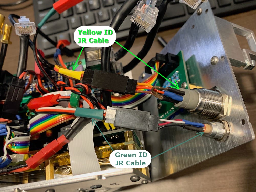
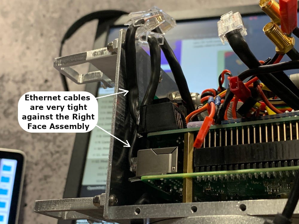
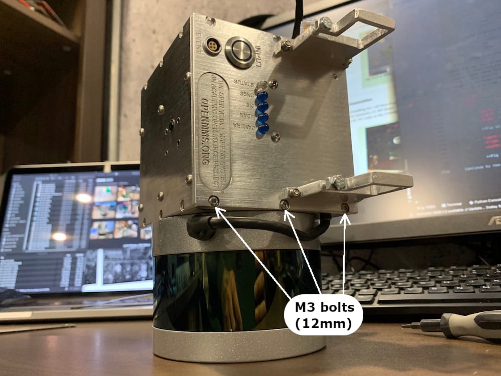
12.4. Attach the Back Face
Caution
The micro-USB port on the Hak5 ethernet switch is only held on the PCB by several small solder joints. Be very careful when plugging and unplugging the USB power cable. THE PORT CAN BE EASILY DAMAGED!
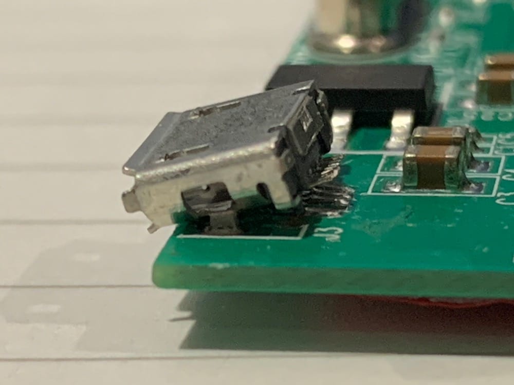
Fig 12.4-1. Damaged micro-USB port on the ethernet switch
Installing the Back Face Assembly within the current Case Assembly requires ten (of the remaining eleven) cables to be connected. To start, connect the micro-USB power cable from the RPi Board to the bottom corner of the ethernet switch (which is mounted on the Back Face Assembly). Next, position the Back Face, so it is in the correct alignment with the sides of the cases, but align its bottom edge near the middle bolt hole on the sides (see figure below). Move the four ethernet cables and the two coaxial GNSS antenna cables towards the Front Face to make room to position the Back Face. The micro-USB power cable for the ethernet switch MUST be positioned behind the INPUT pushbutton (i.e., on the side of the pushbutton that is closer to the Front Face). Then, slowly begin sliding the Back Face, down towards the Bottom Face, while watching to ensure the micro-USB cable stays in the proper position. Pay close attention that NO cables are pinched between the faces of the case or other internal components. Lastly, fasten the Back Face Assembly to the sides and Bottom Face using M3 button-head bolts 12mm in length.
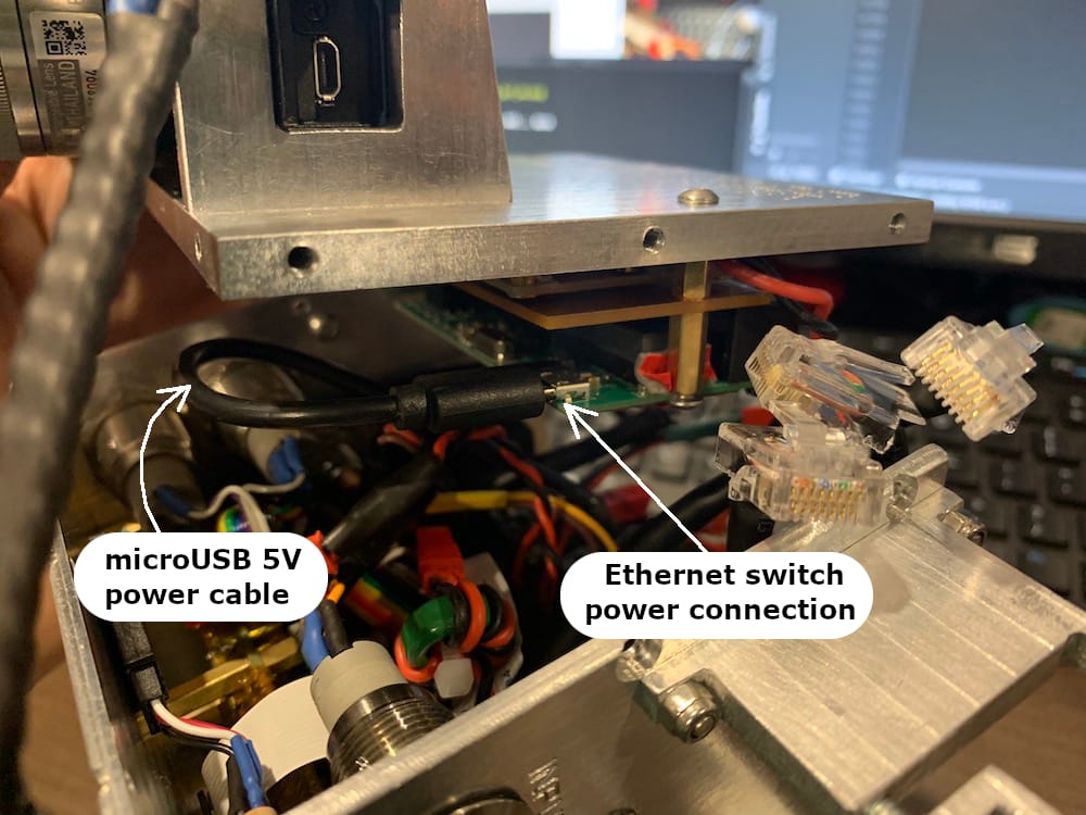
Fig 12.4-2. micro-USB power cable for ethernet switch
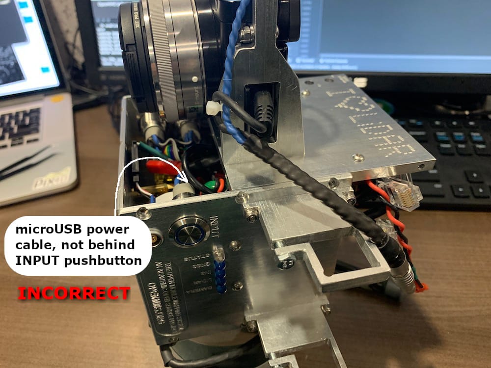
Fig 12.4-3. Back Face aligned with the sides
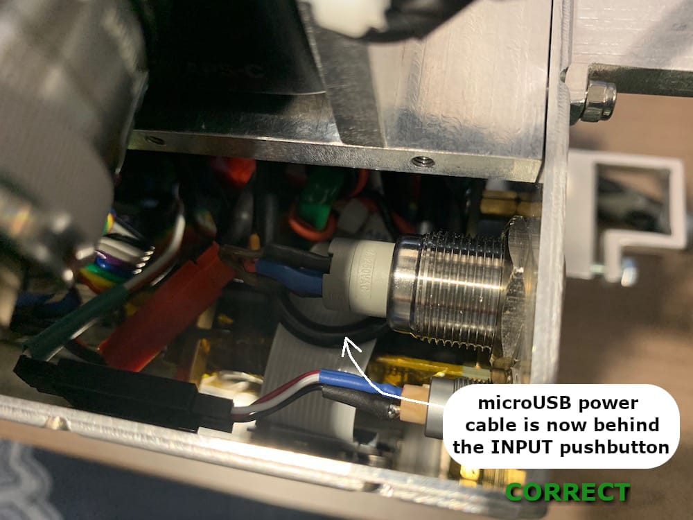
Fig 12.4-4. Position micro-USB cable ‘behind’ the pushbutton
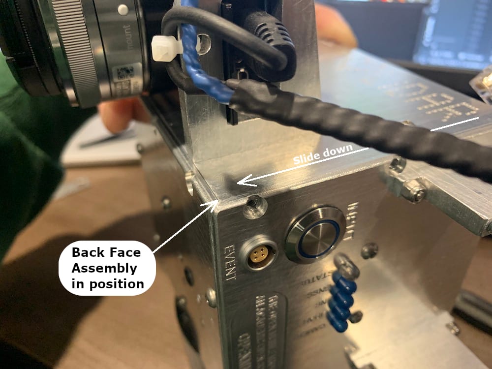
Fig 12.4-5. Back Face in the final position, time to attach
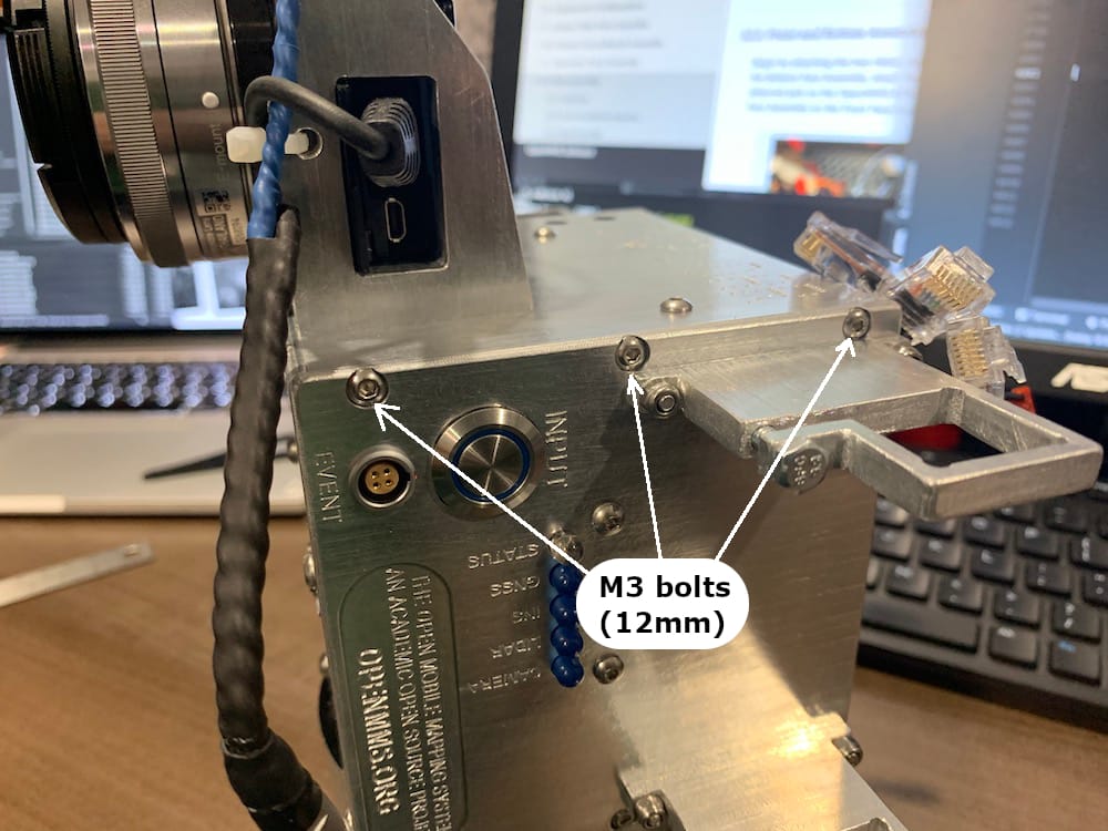
Fig 12.4-6. Fasten Back Face to Right Face
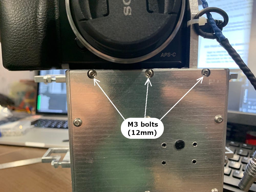
Fig 12.4-7. Fasten Back Face to Bottom Face
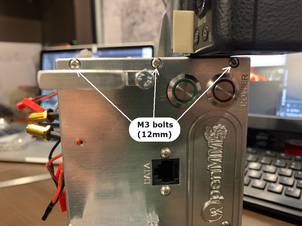
Fig 12.4-8. Fasten Back Face to Left Face
Next, the two internal coaxial GNSS antenna cables need to be installed in their respective positions within the Back Face. Cable 1 goes into the top hole while cable 2 goes into the bottom hole (review Figure 12.3-3). Make sure the hex cable ends are properly aligned with the hex slots machined into the Back Face. On the outside of the case, slide the star washers and locking nuts onto the threaded ends of the coaxial cables and tighten them securely.
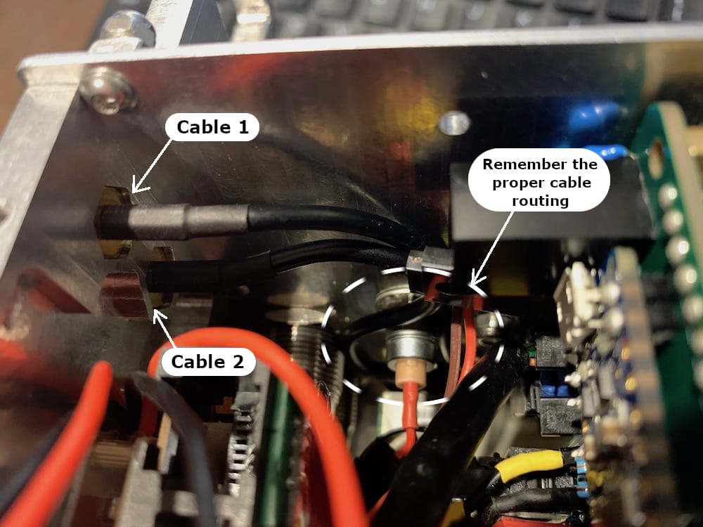
Fig 12.4-9. Coaxial cables positioned in the hex slots
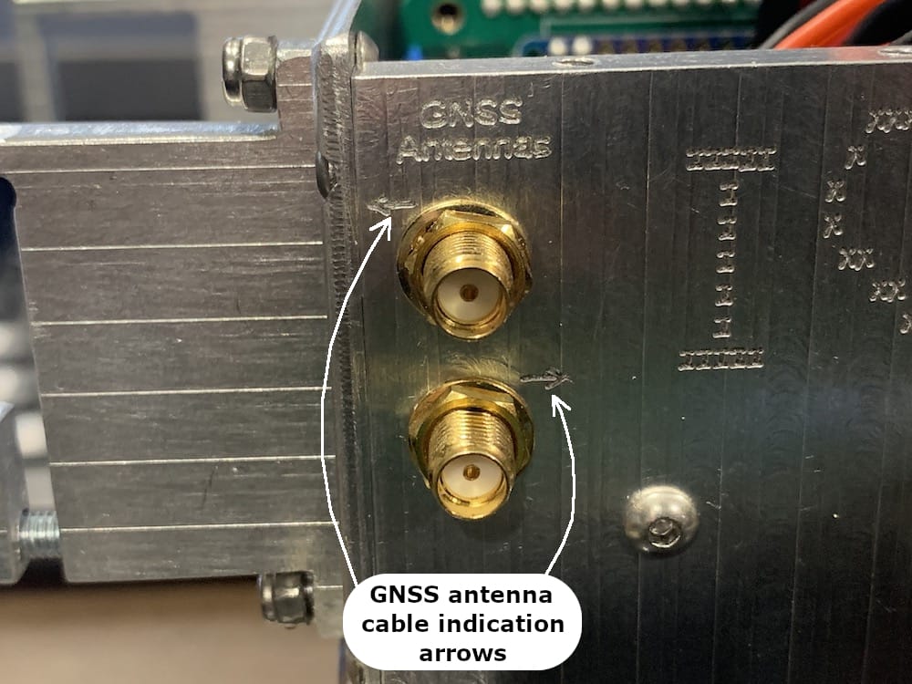
Fig 12.4-10. Coaxial cables secured to the Back Face
Next, the battery (fuse-protected) output power cable from the RPi Board (i.e., green ID 2-wire JST cable) needs to be connected to the INPUT cable on the Matek Systems UBEC Duo (see figure below). The two OUTPUT cables from the UBEC Duo need to be connected to the two SHORT cables on the RPi Board. The OUTPUT 1 (12V) needs to be connected to the short 2-wire JST cable, while OUTPUT 2 (5V) needs to be connected to the short 2-wire JR/Futaba cable. After these three cables have been connected, the cables should be routed ‘behind’ the ethernet switch, then around its left side, and finally tucked neatly between the ethernet switch and the RPi Board (see figure below). Lastly, the four ethernet cables are connected to the four leftmost ports on the ethernet switch. The rightmost ethernet port must be left empty because the aluminum support bracket, attached to the Top Face, occupies the space above this port.
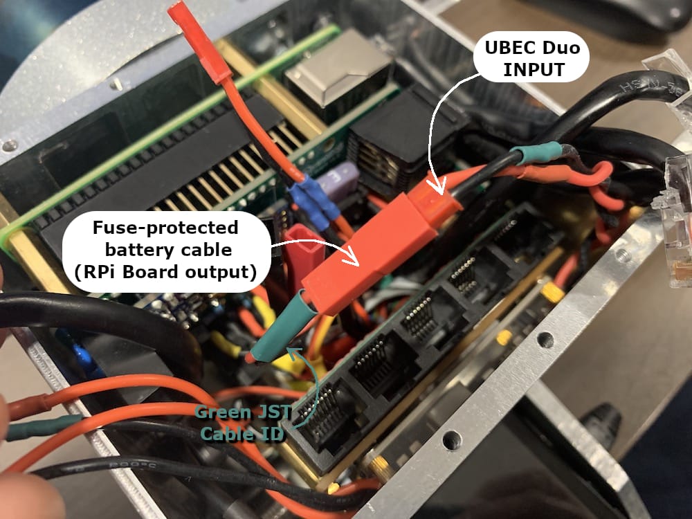
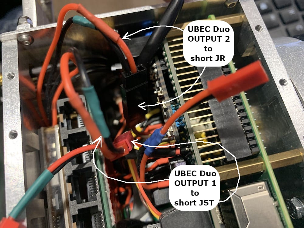
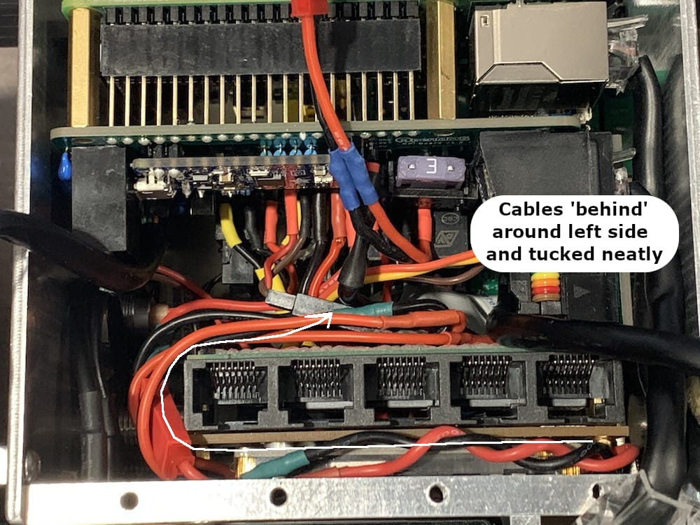
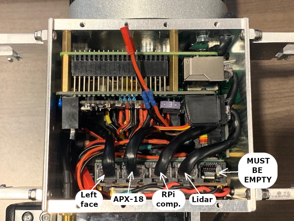
12.5. Attach the Top Face
Installing the Top Face Assembly onto the current Case Assembly is the easiest task in this section. Begin by connecting the Red ID 2-wire JST cable, which is directly connected to the sensor’s power supply, to the cable on the Top Face. Neatly tuck the excess cable between the ethernet switch and the RPi Board, as performed in the previous step. Next, slowly and carefully lower the Top Face onto the Case Assembly. The ethernet cables will likely provide a little resistance to the Top Face being lowered; this is normal as the ethernet cables are designed to fit tight. The six M3 12mm bolts on each of the side faces may have to be loosened slightly for the Top Face to seat on the top of the Case Assembly properly. Additionally, the lidar ethernet cable’s plastic connector may have to be trimmed slightly to provide enough room for the right side support bracket to fit. Before installing the Top Face using the M3 14mm bolts, double-check that the support brackets align with the holes in the side faces. Adjust the support brackets if needed. Lastly, insert the eight M3 14mm long bolts through the Top Face holes, and the two M3 8mm long bolts through the Left and Right Faces, and evenly tighten all the bolts. If the bolts in the side faces needed to be loosened to allow the Top Face to be installed, re-tighten them.
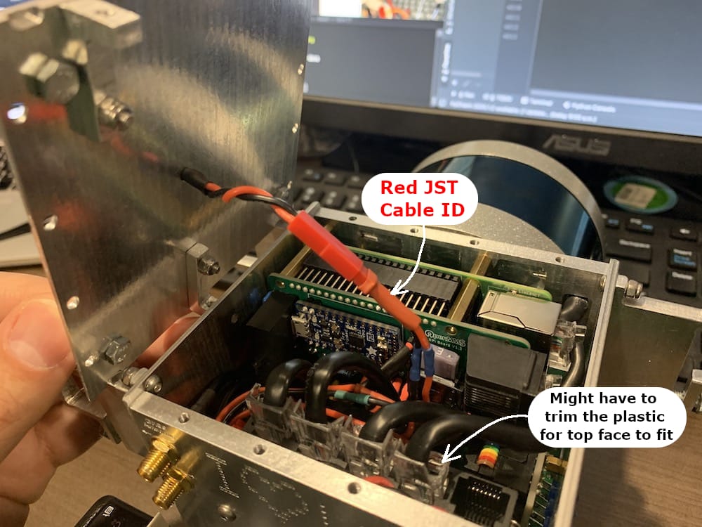
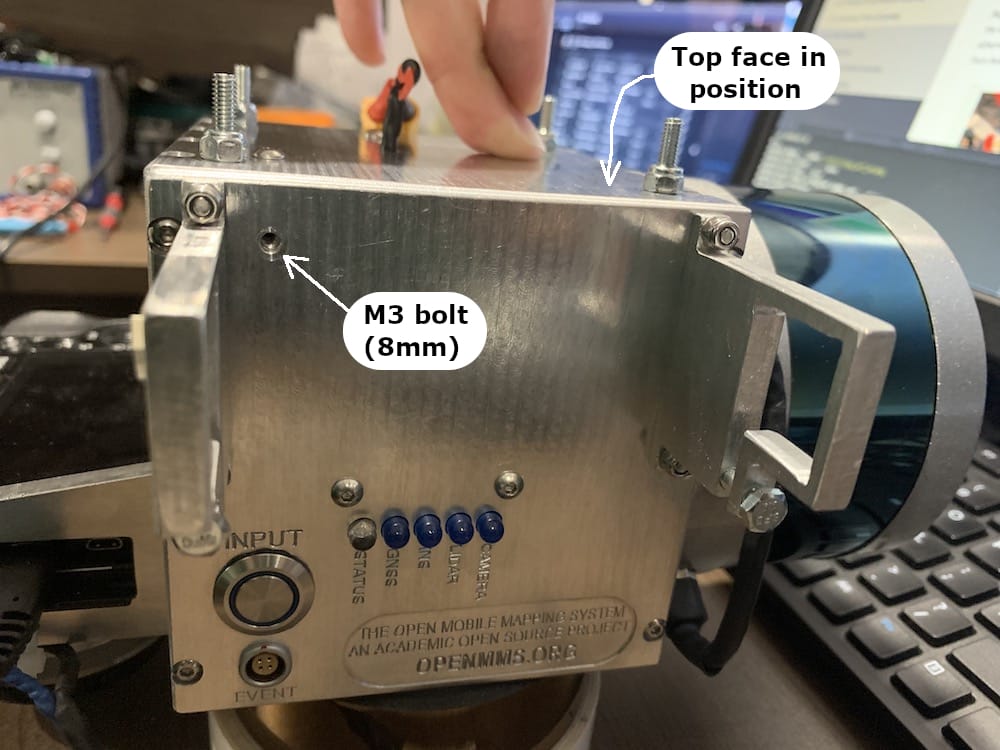
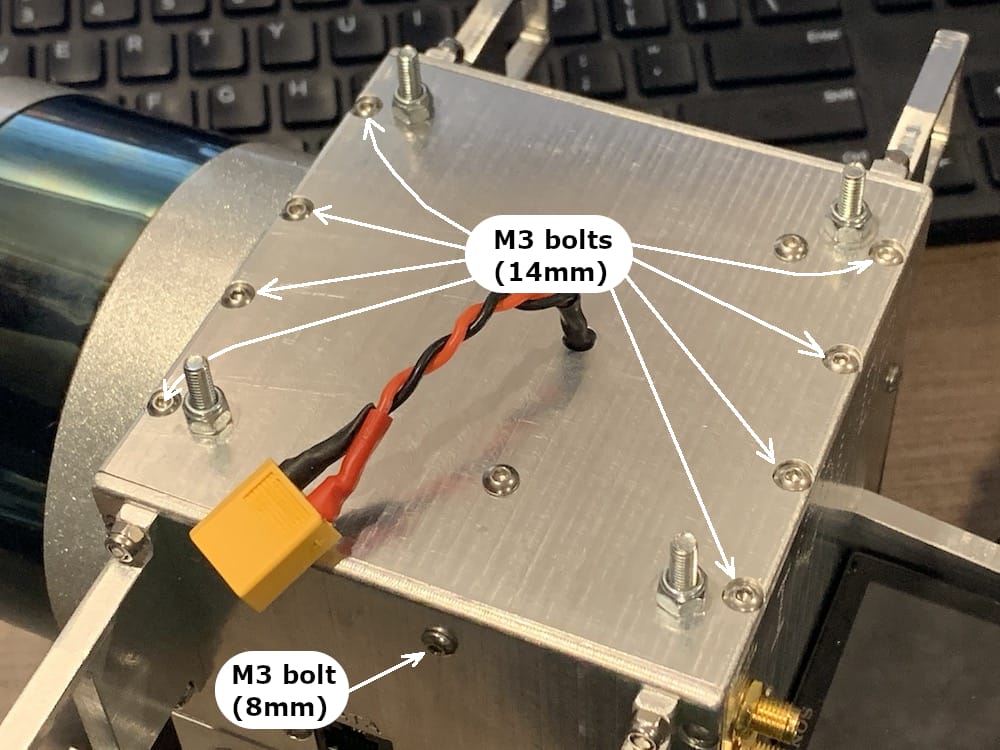
12.6. Connect the Sony A6000 Camera
Before installing the Sony ‘dummy’ battery cable into the A6000 camera, a small rubber/plastic piece must be removed from the battery compartment door (see figure below). This small piece is designed to be removed for this exact purpose (i.e., for powering the camera using an external source). Install the battery into the camera, route the cable through the small opening in the door, close and lock the battery door, and then connect the battery cable to the 9V port on the Left Face of the case. The placement of the camera and the 9V port on the case have been designed to allow adequate access (though tight) to the SD card slot on the camera while leaving the battery cable connected.
The Sony trigger and event cable simply connects to the EVENT port on the Right Face of the case.
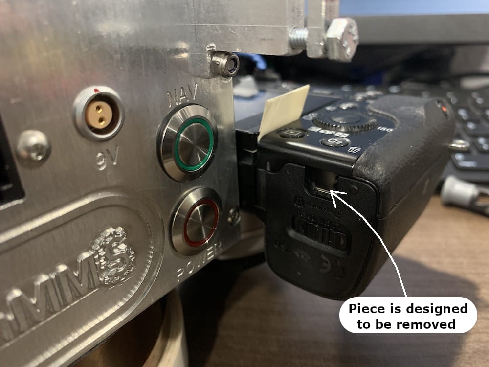
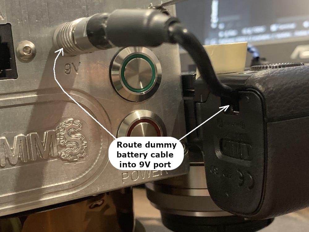
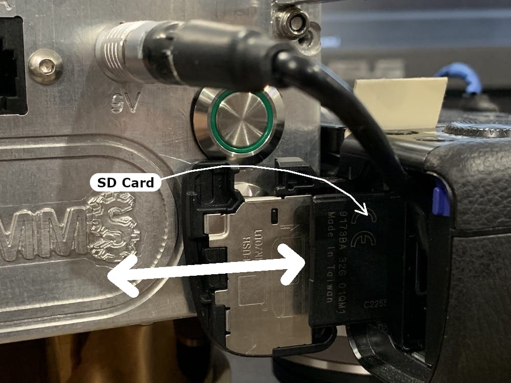
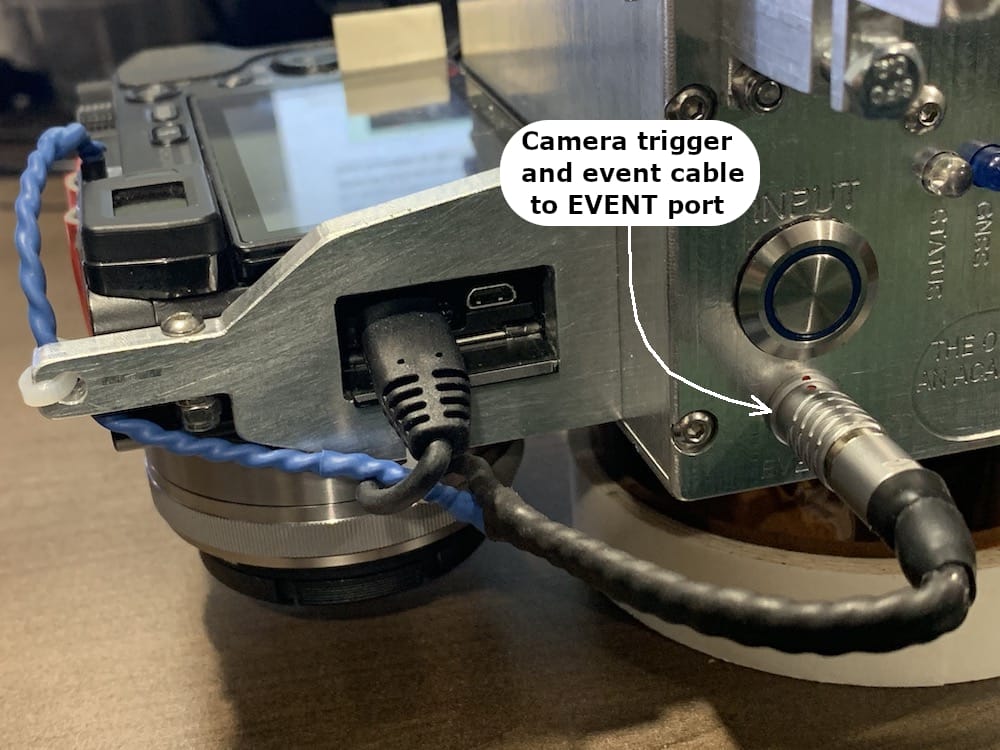
12.7. Connect the GNSS Antenna Arms
Important
The carbon fiber square tubing should slide through the aluminum brackets relatively easily. A small amount of friction is desired, BUT NOT A LOT. If the arms do not slide through easily, it is recommended to file the four inside faces of the aluminum brackets, and NOT THE THIN CARBON FIBER TUBE. Be cautious of the aluminum ‘dust’ created during filing and make sure it does not get into any electronic components.
The two carbon fiber GNSS antenna arms have been designed to be lightweight, strong, and easily installed and removed from the case. The arms are NOT identical and therefore need to be installed in a specific way. The arm that has the antenna cable running its entire length is installed through the aluminum GNSS brackets on the Left Face of the case with the GNSS antenna pointing towards the lidar sensor. On the left side only, the GNSS antenna cable’s SMA connector must be carefully inserted through each aluminum bracket before the carbon fiber arm is inserted. The arm with the GNSS antenna cable exiting from the side of the tubing is installed through the GNSS brackets on the Right Face of the case with the GNSS antenna pointing towards the Sony camera. The lidar side GNSS antenna cable is attached to the top threaded coaxial connector on the Back Face. Therefore, the camera side GNSS antenna cable is attached to the bottom threaded coaxial connector on the Back Face. There are small engraved arrows beside the threaded coaxial connectors that point to the GNSS antenna cable that attaches to each respective connector (see Fig 12.4-10). Finally, tighten the M4 bolt on each of the aluminum brackets to secure the GNSS antenna arms to the case. BE CAREFUL NOT TO OVER-TIGHTEN THESE BOLTS AS THIS MAY DAMAGE THE CARBON FIBER TUBES.
Warning
It is recommended that the GNSS antenna arms be inserted ~5mm past the end of the 2nd aluminum bracket on each side. Over-inserting the GNSS antenna arms help prevent the open end of the square carbon fiber tubes from being cracked or damaged when the aluminum brackets are tightened. For repeatable installations of the GNSS antenna arms, reference marks should be made on each arm.
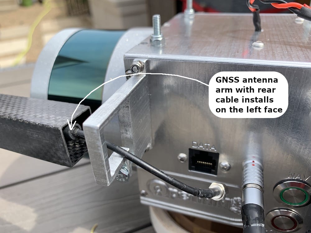
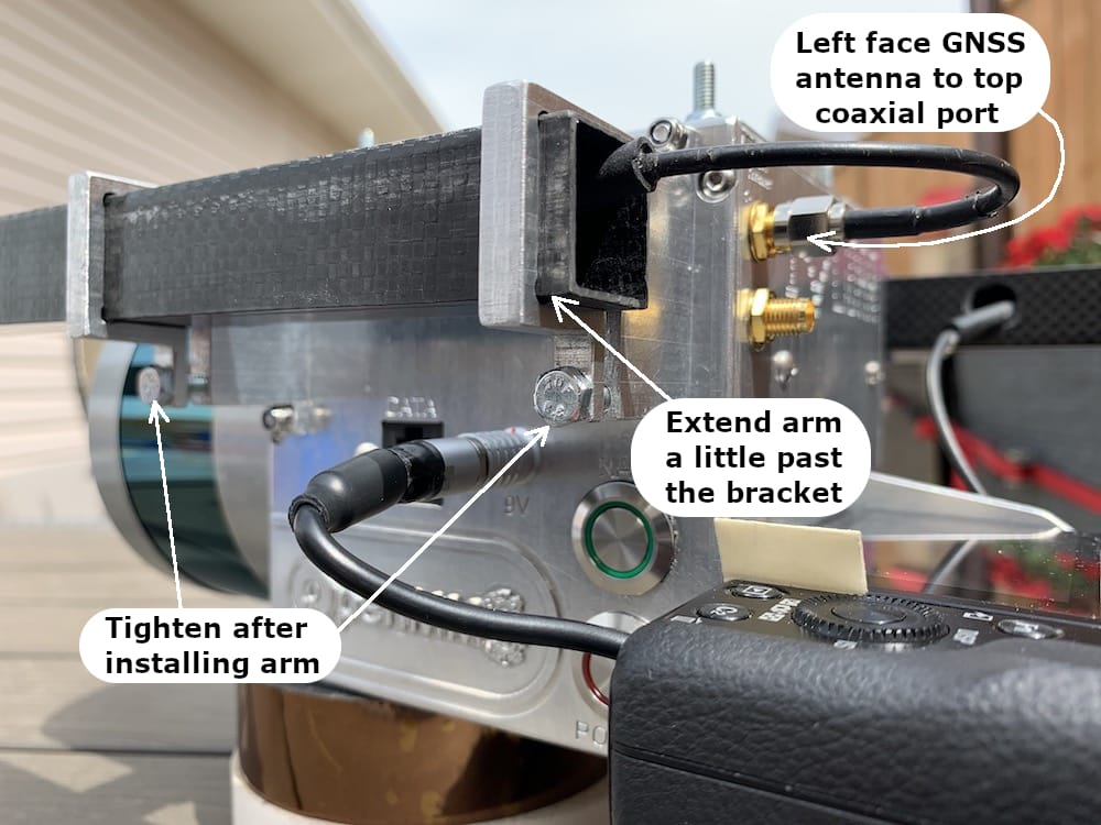
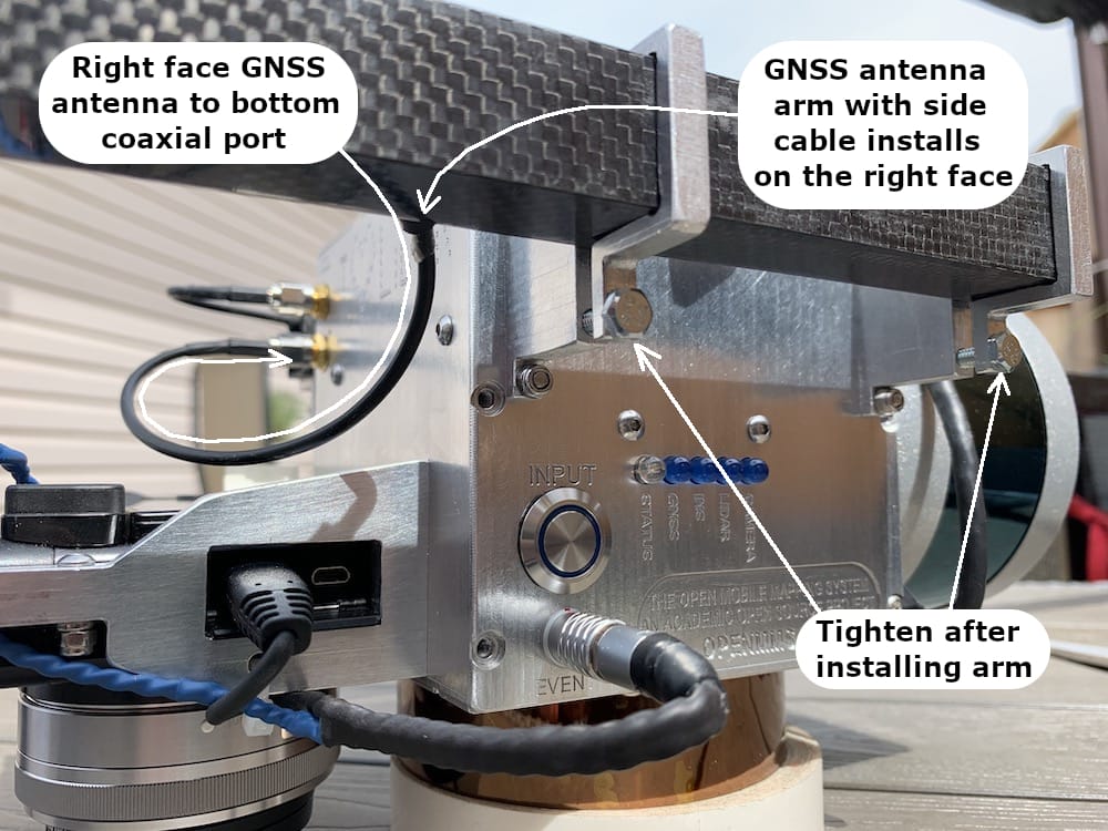
12.8. Completed OpenMMS V1.3 Sensor
The final size and weight properties of the OpenMMS V1.3 sensor are:
162cm x 28cm x 20cm
25cm x 20cm x 15cm (without GNSS arms and antennas)
2.5 kg (VLP-16) or 2.3 kg (VLP-16 Lite) or 2.4 kg (MID-40)
CONGRATULATIONS!
YOU HAVE NOW FINISHED BUILDING YOUR OPENMMS V1.3 SENSOR! HOPEFULLY, THE EXPERIENCE WAS EDUCATIONAL AND MEMORABLE. WE WOULD ENJOY HEARING FROM YOU ABOUT YOUR THOUGHTS AND COMMENTS (GOOD AND BAD) ON THE PROJECT.
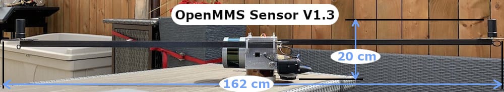
Fig 12.8-1. Side view of the OpenMMS V1.3 Sensor (VLP-16)
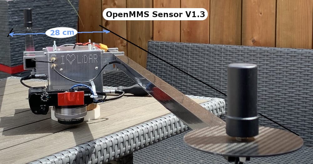
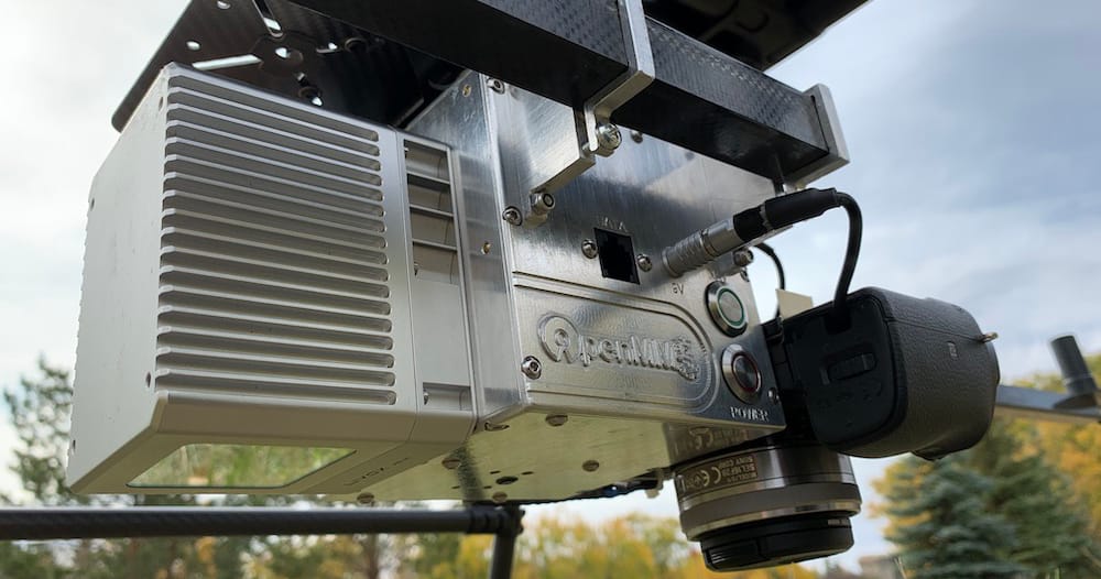
12.9. Calibrating the GNSS Lever-arms
This section presents the first of three calibration procedures that need to be performed on the OpenMMS sensor. This procedure aims to precisely estimate the offsets (i.e., distances) between the phase centers of the GNSS antennas and the origin of the lidar sensor’s coordinate system. These offsets are known as lever-arms, and are a set of three orthogonal distances, within a specific frame of reference, between the points of interest. As neither the phase center of a GNSS antenna nor the lidar sensor’s origin can be physically observed, precisely estimating the lever-arms can be a difficult task.
Tip
It is recommended to occasionally re-perform the GNSS lever-arm calibration procedure, to ensure that the lever-arm offset values are remaining constant.
The OpenMMS lever-arms calibration procedure utilizes an optical triangulation technique, commonly referred to as theodolite intersection. As the name implies, a theodolite (i.e., optical angular measuring instrument) is required to perform the calibration procedure. A modern total-station instrument can, of course, be substituted for a theodolite. As only horizontal and vertical angles are directly observed using the total-station, the derived offsets’ scale still needs to be defined. The scale is defined by establishing a short reference baseline (i.e., 2 points on the ground) and measuring the slope distance using a tape measure. Then the fully assembled OpenMMS sensor is positioned in a stationary pose on one side of the baseline, approximately perpendicular from the midpoint of the baseline, see Figure 12.9-1.
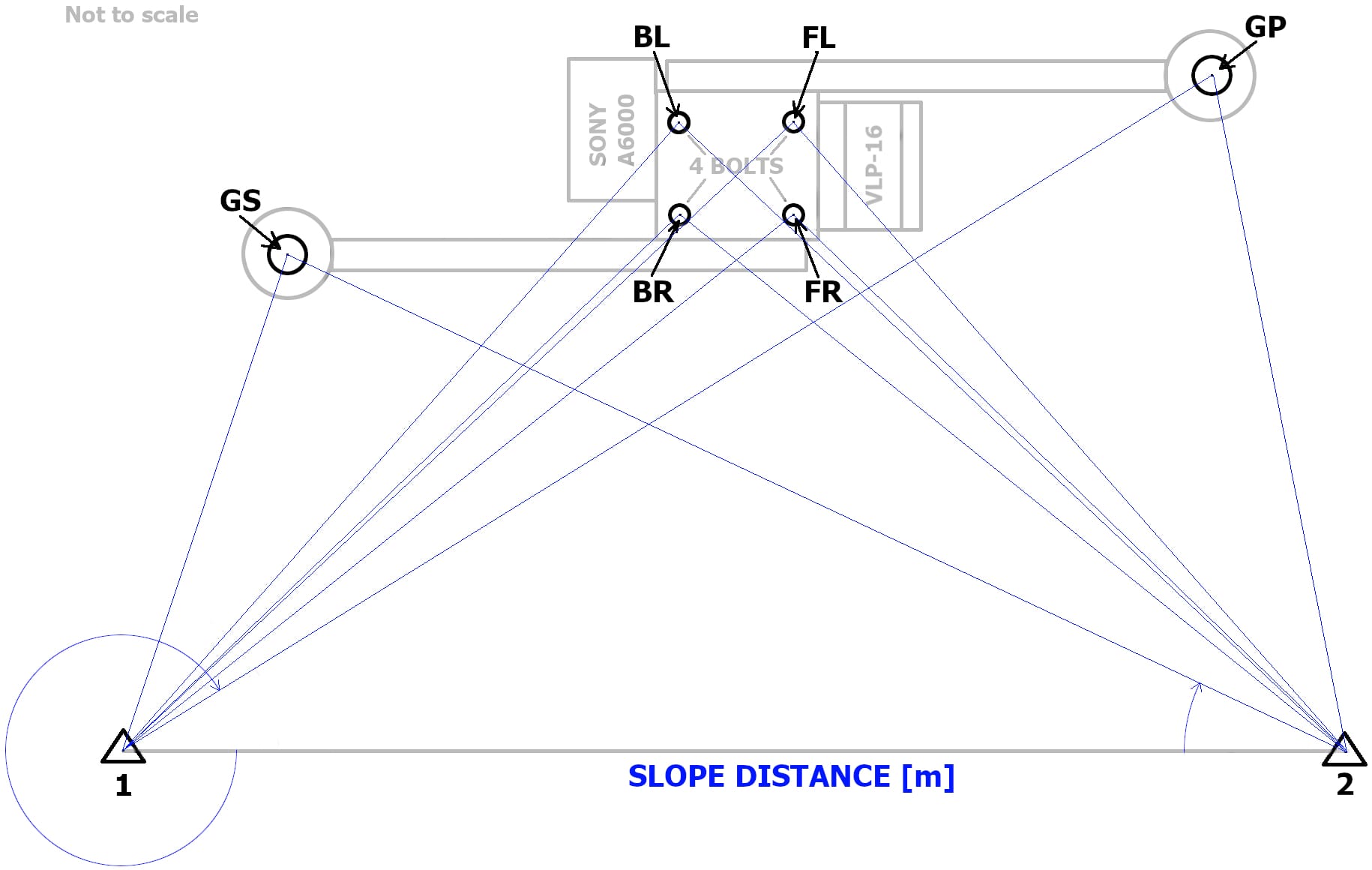
Fig 12.9-1. OpenMMS GNSS lever-arms calibration layout

Fig 12.9-2. Total station observing OpenMMS sensor from BL pt. 1
Warning
It is vital that the OpenMMS sensor remains perfectly stationary during the entire lever-arms calibration procedure! The orientation of the OpenMMS sensor with respect to the baseline is not crucial as the Excel spreadsheet calculations account for any orientation differences. The orientation shown above is recommended for simplicity.
The sighting location for each of the observation points on the OpenMMS sensor includes the top-center of the Trimble AV14 GNSS antennas (see Figure 12.9-3), and the top-center of the four M4 mounting bolts extending through the Top Face of the OpenMMS case (see Figure 12.9-4). The occupation points for the theodolite/total-station are the baseline points 1 and 2, respectively. The backsight point for each occupation is the center of the unoccupied baseline point, directly observed on the ground.
To simplify the observation procedure and the necessary calculations, a Microsoft Excel spreadsheet template is provided that clearly and concisely defines what observations need to be made to precisely estimate the GNSS lever-arm offsets. See the OpenMMS Applications section in the OpenMMS Software documentation to download the Excel template. The following figure illustrates the layout of the Excel template. All the yellow-colored cells need to be populated with the observations made during the calibration procedure. Once all observations have been entered, the black boxes at the bottom of the template will display the precise estimates for the GNSS lever-arm offsets. These values then need to be entered into the firmware of the Applanix APX-18 and saved. See Figure 8.6-19a or Figure 8.6-19b for details on where to enter the precise lever-arm offset estimates within the APX-18 firmware.

Fig 12.9-5. OpenMMS GNSS Antenna Lever-arms MS Excel Template
Pay close attention to cells C12, C13, C14, and E16 in the above figure. These cells need to be populated with the necessary non-angular observations. Cell C12 requires the slope distance between baseline points 1 and 2, as measured with a hand tape, to be entered in units of meters. Cell C13 requires the height of the four bolts extended out of the top face of the case. This measurement needs to be made from the top face to the threaded end of the bolt (it is assumed that all bolts will have exactly the same measurement from the top face). Cell C14 requires the offset from the top of the GNSS antenna to its phase center location. For Trimble AV14 antennas the offset is ~0.03m. If different GNSS antennas are used, it is the reader’s responsibility to enter the proper phase center offset from the top of their respective GNSS antenna. The template assumed that both GNSS antennas have the same offset. Lastly, cell E16 requires the Height of the Instrument (HI) to be entered. This measurement is from the baseline point 1 to the observational axis (i.e., trunnion axis) of the theodolite/total-station. The instrument should have a reference mark that allows this measurement to be easily made. One quality assurance metric is incorporated within the Excel template. Cells E46-E52 report the difference in the Z coordinate for the observation points on the OpenMMS sensor. The values in this range of cells should be approximately zero (i.e., 0.000m).
Attention
The OpenMMS GNSS lever-arms calibration procedure assumes that the theodolite/total-station instrument being used to conduct the observations is appropriately calibrated. If the user is unsure about the accuracy/calibrated state of the instrument, the angular observations should be made using both faces of the instrument, and then a reduced singular observations entered into the Excel template.
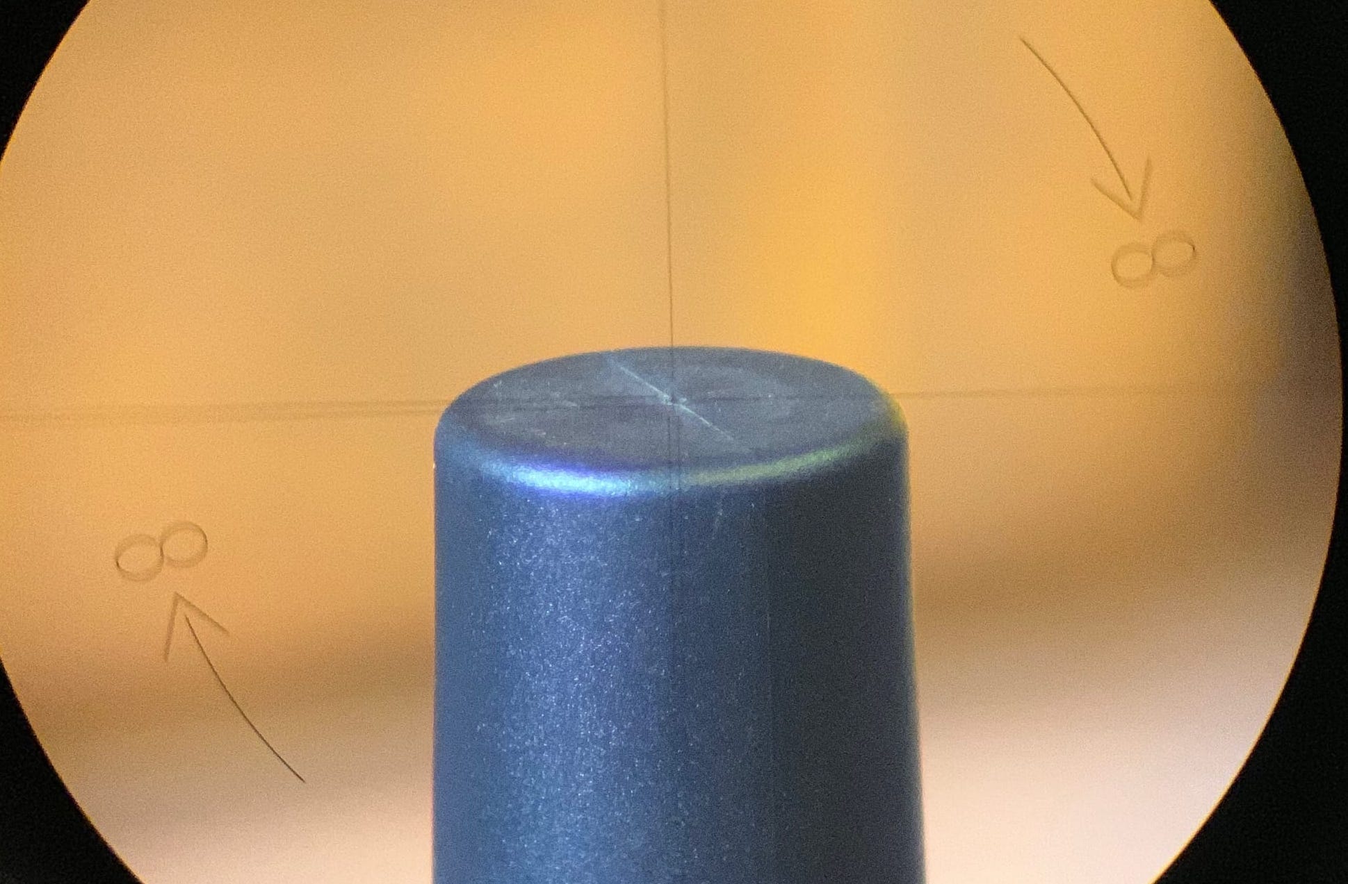
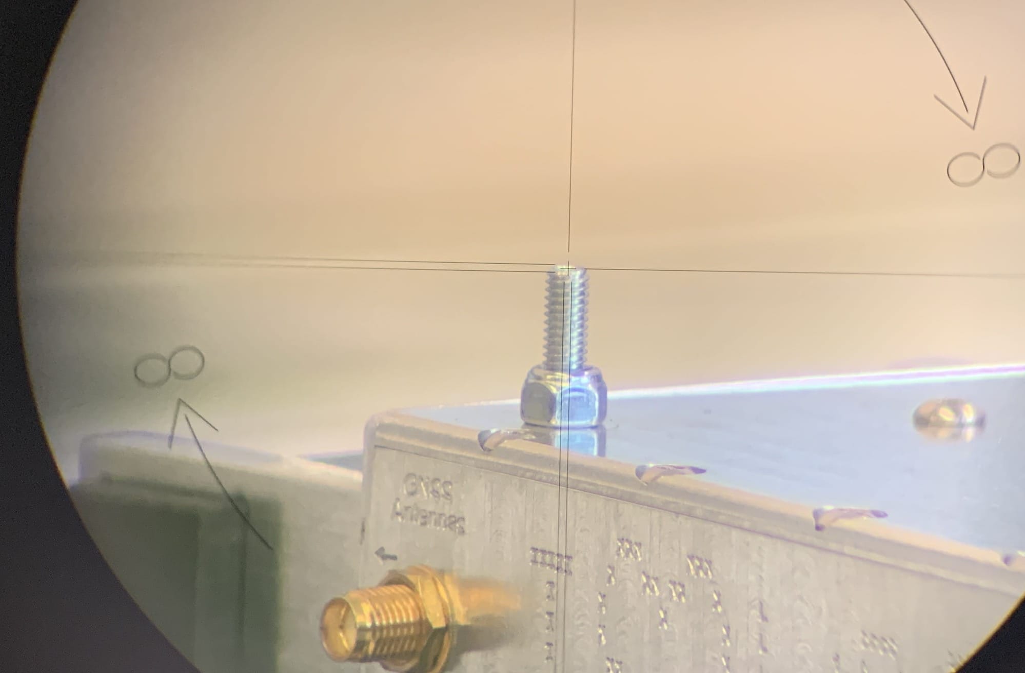
13. Sensor Operations
13.1. Overview
Attention
The alignment of the OpenMMS sensor with respect to the vehicle frame it is installed on is very important to understand. The side of the OpenMMS sensor where the Sony A6000 camera is mounted, referred to as the Back Face during the previous manufacturing and assembly steps, needs to be installed, so it points in the nominal forward direction of the vehicle (e.g., UAS, automobile, backpack, etc.). Expressed in a different way, the lidar sensor needs to point towards the backward/reverse direction of the vehicle. See the following figure for clarification.
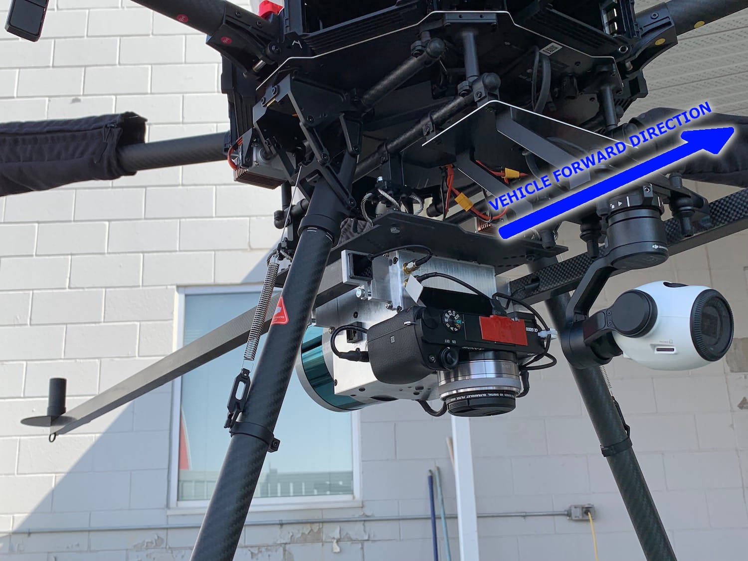
Fig 13.1-1. OpenMMS Sensor orientation with respect to a UAS vehicle frame
The OpenMMS V1.3 sensor has been designed to be easy to operate using a simplistic hardware User Interface (UI). Additionally, some sensor settings can be changed/reconfigured, at any time, by connecting an ethernet cable from a computer to the DATA port on the sensor, and then using a web browser application.
13.2. Sensor Power Supply
The sensor’s primary voltage regulator circuit utilizes the Matek Systems UBEC Duo component. The input voltages supported by this component can range from 7V - 26V. However, because the lidar sensor integrated into the OpenMMS sensor require a 12V supply, a minimum input voltage of 12V is needed as the UBEC Duo does not provide any voltage step-up features. The OpenMMS V1.3 sensor supports a 12V to 26V power supply, and uses an XT-60 connector. A typical power supply option is the use of a 4-cell (4S) Lithium Polymer (LiPo) battery commonly for RPAS/UAS/UAV/Drone operations, or a typical automotive 12V lead-acid battery for vehicular operations.
13.3. Sensor Power Up
There are three ON/OFF switches that need to be set to ON to power up the OpenMMS sensor. The switches should always be turned ON in the following order:
POWER (Red) pushbutton on the Left Face, press it in until it latches and the ring LED turns ON.
- Wait until the STATUS LED on the Right Face starts to quickly flash red, then green, then blue.Sony A6000 camera’s ON/OFF switch, the display screen will turn on.
- If photos are not required as part of the data collection, then this can stay OFF.NAV (Green) pushbutton on the Left Face, press it in until it latches and the ring LED turns ON.
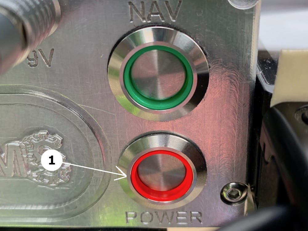
Fig 13.3-1. POWER pushbutton
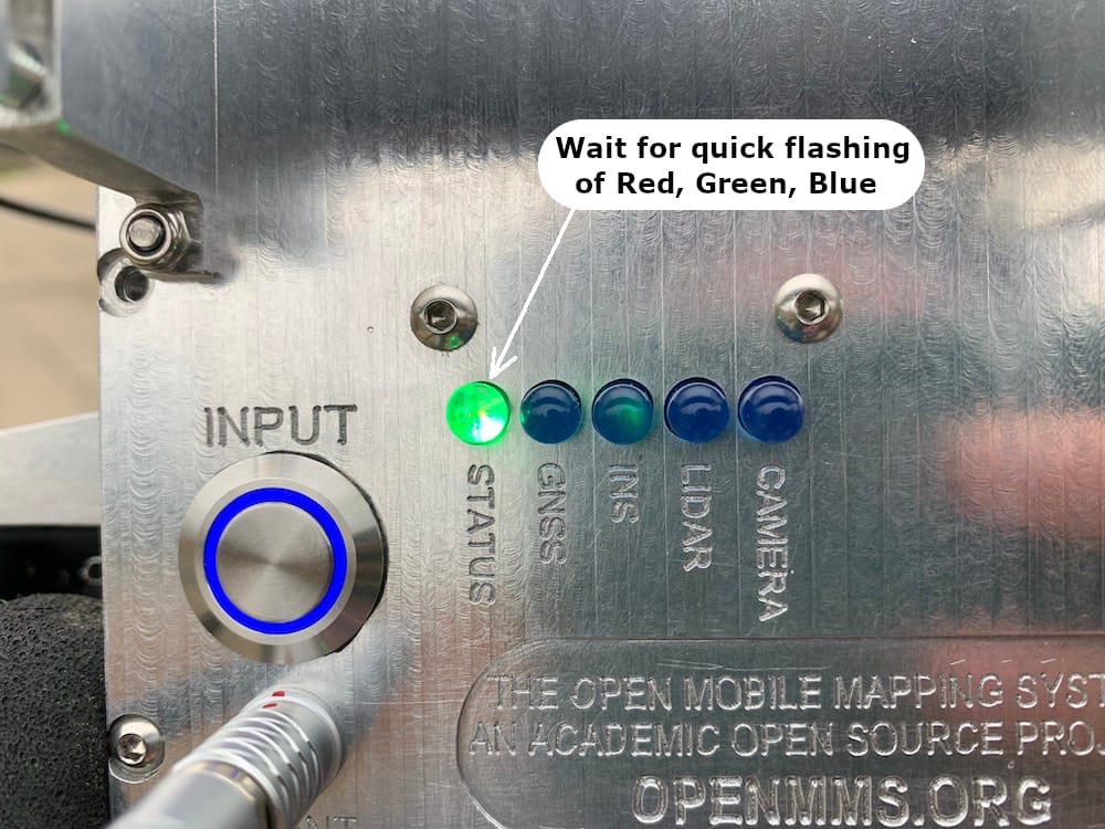
Fig 13.3-2. Wait for STATUS LED
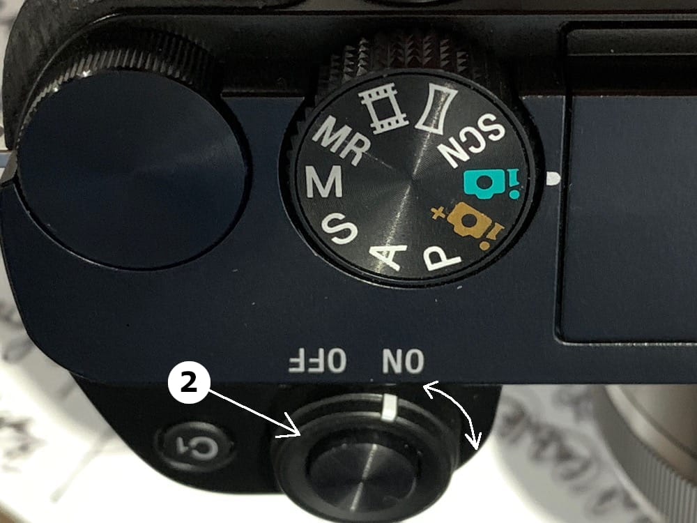
Fig 13.3-3. Sony A6000 ON/OFF
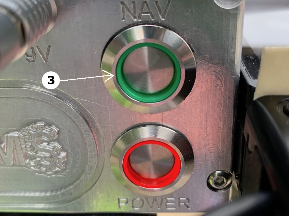
Fig 13.3-4. NAV pushbutton
The OpenMMS sensor is ready to begin collecting digital mapping data when all three ON/OFF switches have been turned ON, the STATUS LED is solid Green, and the GNSS and INS LEDs are blinking at the same time, once every second (i.e., at 1 Hz). How to initialize the GNSS-INS sensor will be discussed in an upcoming section.
13.4. INPUT Pushbutton and STATUS LED
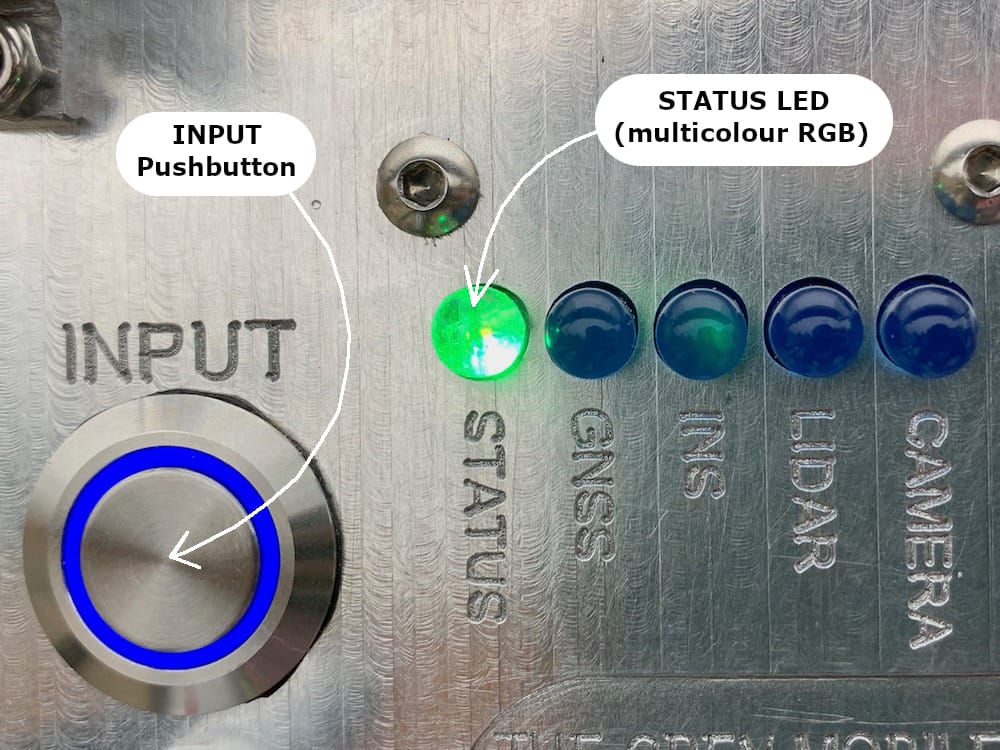
Fig 13.4-1. INPUT Pushbutton and STATUS LED on the Right Face
The INPUT pushbutton on the OpenMMS sensor V1.3, is a momentary button (i.e., does not latch) that the operator uses to instruct the sensor to perform an operation. Currently, there are a total of four operations that can be performed. The chosen operation is indicated by the STATUS LED flashing from solid Green to Blue a set number of times while the operator is pressing in and holding the INPUT pushbutton. When the operator releases the INPUT pushbutton after witnessing the desired number of Blue STATUS LED flashes, the OpenMMS sensor begins the respective operation. The timing of when the operator releases the INPUT pushbutton determines what operation the sensor performs. This concept may be difficult to understand by only reading this documentation, but will be easily understood in practice.
As a crude analogy, think of the STATUS LED as being like a computer monitor, pressing in and holding the INPUT pushbutton as being like moving a computer mouse around the monitor, and then releasing the INPUT pushbutton as being like clicking the mouse button.
The following table indicates how the STATUS LED, and INPUT pushbutton are used to execute one of the four possible operations when the sensor is in its Standby Mode:
Table H19: OpenMMS Sensor Operations
Description of the Operation
INPUT Pushbutton State
STATUS LED Before
Execute Operation By
STATUS LED After
Sensor is Ready to Go (Standby Mode)
Not pressed
Solid Green
Not Applicable
Not Applicable
Lidar and Photo observations started
Press in and hold
1 Blue Flash
Releasing INPUT within 1 sec
Solid Blue
Photo only observations started
Press in and hold
2 Blue Flashes
Releasing INPUT within 1 sec
Solid Blue
Raspberry Pi Computer safely shutdown
Press in and hold
3 Blue Flashes
Releasing INPUT within 1 sec
Turns Off (still faint)
ERASE ALL stored data on the Raspberry Pi
Press in and hold
4 Blue Flashes
Releasing INPUT within 1 sec
Green Flashing then Solid Green
Return to Standby Mode, no op. executed
Press in and hold
Red then Blue then Green Flash
Releasing INPUT within 1 sec
Solid Green
Stop data collection
Press in and hold
Solid Blue
Continue holding until LED Off
Green Flashing then Solid Green
The STATUS LED will also be observed displaying several other solid and flashing colors during certain times while operating the OpenMMS sensor. The following table provides a summary of the STATUS LED colors.
Table H20: OpenMMS STATUS LED Indications
STATUS LED Displays
Description
Quick Red, Green, Blue Flashes
Raspberry Pi computer booting up (shows LEDs are functional)
Quick White Flashes
Indicates Raspberry Pi camera video will be recorded
Solid Green
Standby Mode
Solid Blue
Data Collection Mode
Slow Green Flashes
Data file(s) are being created or safely closed
Slow White Flashes to Solid White
Raspberry Pi camera video being converted to MP4
Quick Red Flashes
WARNING: UTC time not set or data couldn’t be erased
Multicolor flashes to Solid Red
ERROR: Lidar and/or real-time Nav. data file failed
13.5. GNSS and INS LEDs
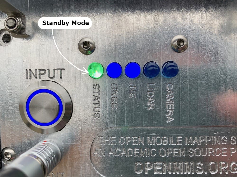
Fig 13.5-1. GNSS and INS LEDs illuminated
The GNSS and INS LEDs are controlled directly by the Applanix APX-18 GNSS-INS sensor. According to Applanix APX-18 Hardware Integration Manual, the GNSS and INS LEDs behave as follows:
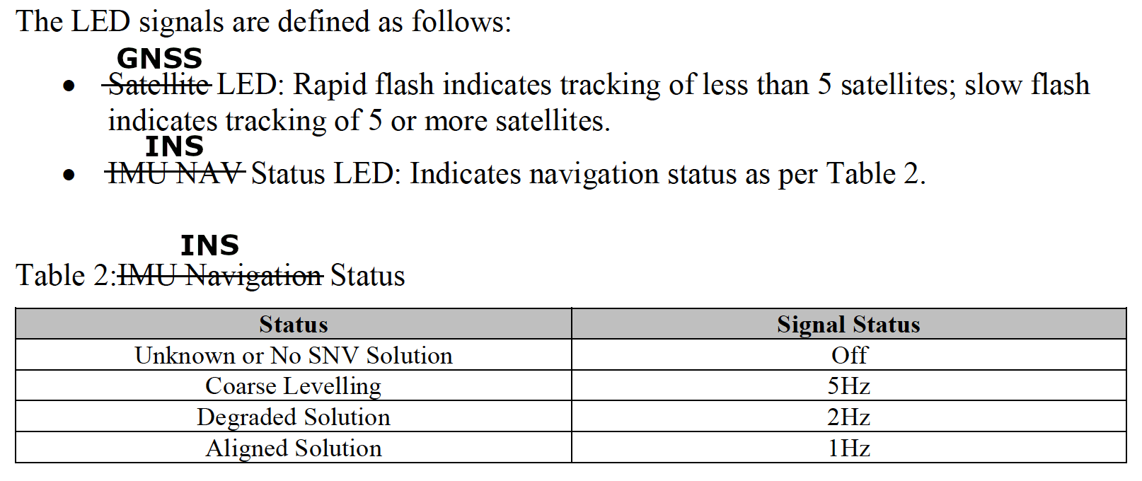
Fig 13.5-2. APX-18 GNSS and INS LED Status (Source: Applanix)
Important
Refer to the complete set of documentation provided by Applanix, or contact their Technical Support team for further details.
13.6. LIDAR and CAMERA LEDs
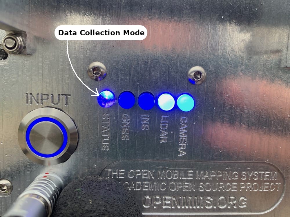
Fig 13.6-1. LIDAR and CAMERA LEDs illuminated
The LIDAR LED is connected directly to the same power circuitry used to provide power to the lidar sensor. The LIDAR LED simply indicates if power is being provided to the lidar sensor or not. Once the lidar sensor is powered on, there is a small time delay before lidar observations begin being stored to a data file onboard the Raspberry Pi (i.e., once the STATUS LED turns Solid Blue, lidar data is being stored).
The CAMERA LED is connected directly to the Adafruit Trinket Pro’s (i.e., the intervalometer’s) output pin 13. The benefit of using pin 13 is that it automatically powers on and off (thereby flashing the CAMERA LED) when the intervalometer is booting up. A user will notice the CAMERA LED flashing quickly and seemingly random when the OpenMMS sensor is first started. The CAMERA LED’s flashing at startup is done intentionally to indicate to the user that the CAMERA LED is functional. However, suppose the Sony A6000 camera is turned on and connected to the trigger and event cable. In that case, the camera will take a photo(s) during the bootup stage of the intervalometer. Hence, the OpenMMS sensor bootup sequence requires the POWER pushbutton to be turned on BEFORE the Sony A6000 camera is turned on. Once the sensor is completely turned on and enters data collection mode, the CAMERA LED will flash whenever the command is sent to the camera to take a photo.
13.7. Sensor Shut Down
Shutting down the OpenMMS sensor follows the same steps as powering up but completed in the reverse order.
NAV (Green) pushbutton on the Left Face, press it in to unlatch, the ring LED turns OFF.
Sony A6000 camera’s ON/OFF switch, the display screen will turn OFF.
- Sometimes the camera will take another photo just before it powers off, be sure to note if this occurs.Press and hold the INPUT pushbutton and wait for 3 quick Blue flashes of the STATUS LED, then let go.
- Wait for the STATUS LED to turn OFF (it will still be dimly lit), then wait approx. 5 sec before continuing.POWER (Red) pushbutton on the left face, press it in to unlatch, the ring LED turns OFF.
13.8. Magnetometer Calibration
Applanix recommends performing a Magnetometer Calibration procedure before collecting mapping data. According to the Applanix documentation, the calibration procedure can be completed as follows:
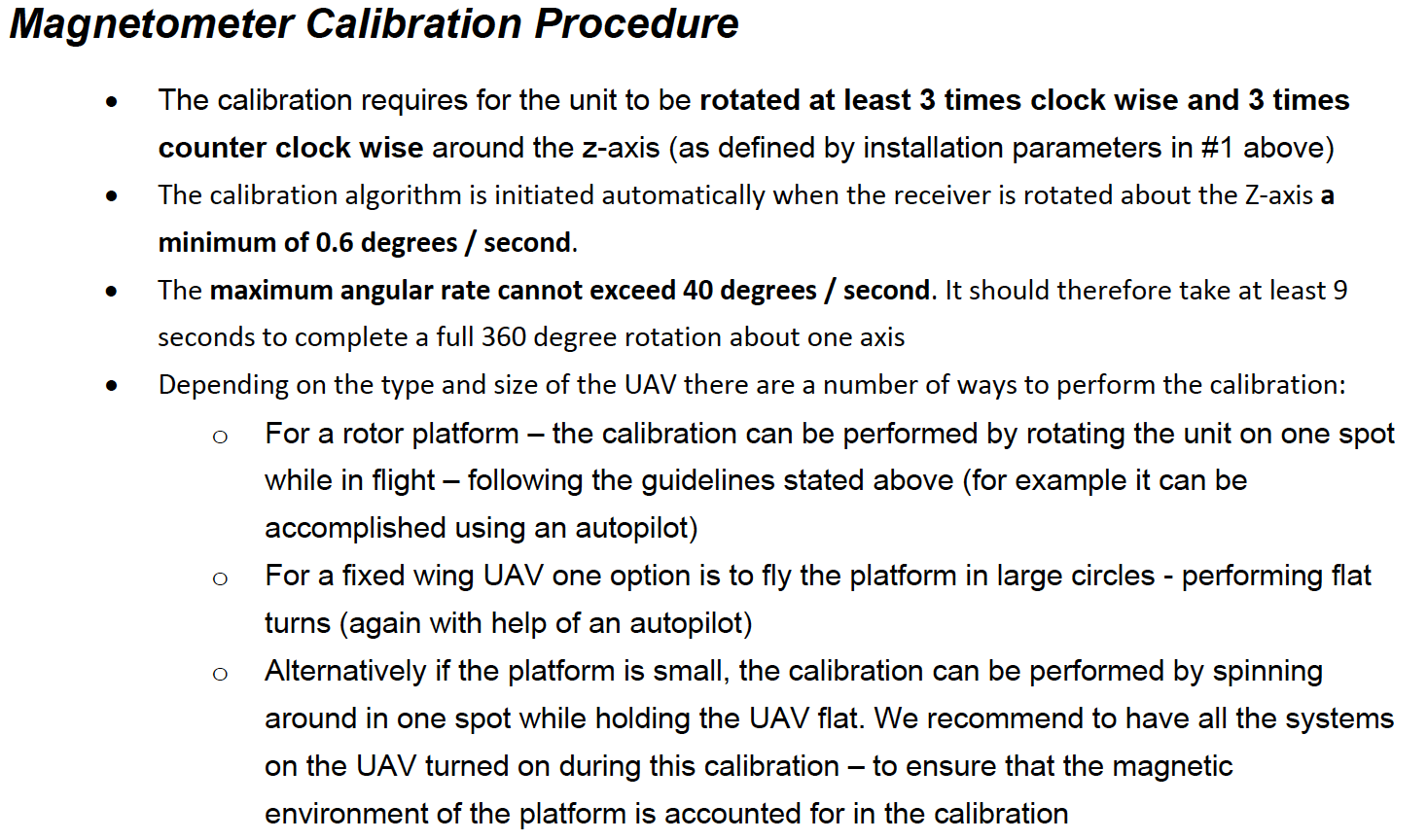
Fig 13.8-1. Applanix Magnetometer Calibration Procedure (Source: Applanix)
Important
Refer to the complete set of documentation provided by Applanix or contact their Technical Support team for further details.
13.9. INS Initialization
Before starting to collect lidar observations or photos from the OpenMMS sensor, the APX-18 needs to be in the Aligned INS state/solution. An Aligned state is indicated by the INS LED flashing at a rate of once per second (1 Hz). See Figure 13.5-1 for reference. Theoretically, with the dual GNSS antennas on the APX-18 it could achieve an Aligned solution by remaining stationary while observing enough GNSS satellites. However, an Applanix recommended approach to achieving an Aligned solution (presented for the APX-15 GNSS-INS sensor) is as follows:
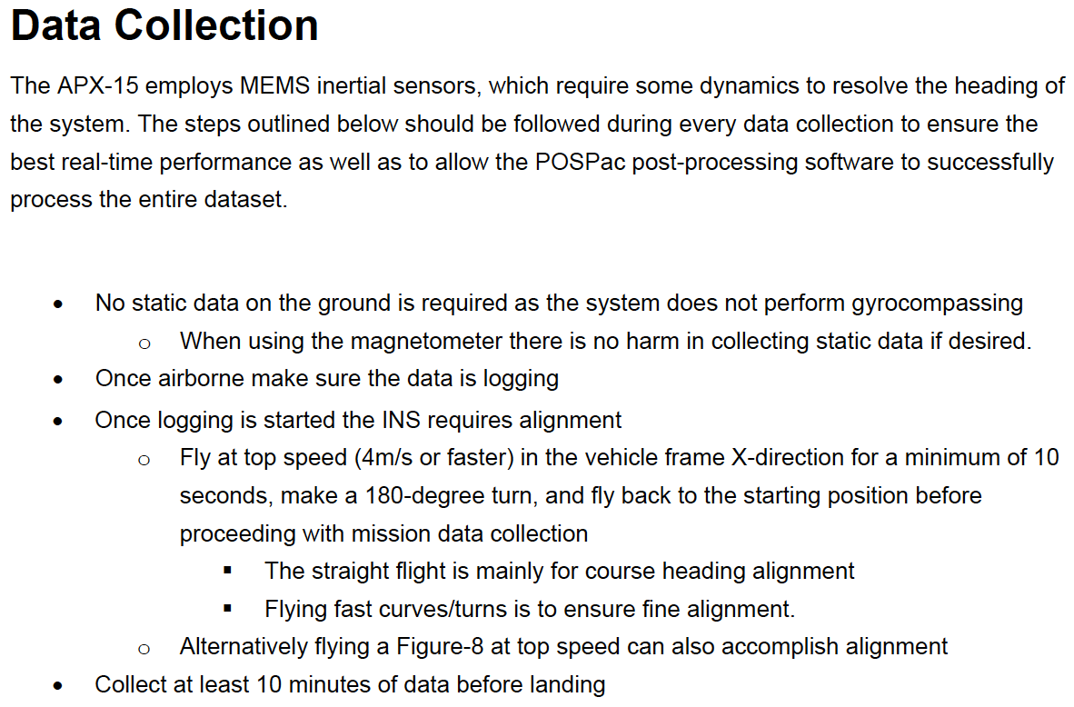
Fig 13.9-1. Applanix INS Initialization Procedure (Source: Applanix)
Important
Refer to the complete set of documentation provided by Applanix or contact their Technical Support team for further details.
13.10. Access the Raspberry Pi (RPi)
Warning
The reader’s computer needs to be physically connected to the OpenMMS sensor using an ethernet cable and assigned an appropriate static IP address and subnet mask to successfully connect to the Raspberry Pi computer. An IP address of 192.168.1.23 and a subnet mask of 255.255.255.0 are recommended.
As discussed in section 8.4, the Raspberry Pi computer provides the user with a Web-based User Interface (WebUI) to access the camera settings and the mapping data files stored within its filesystem. After completing a data collection campaign, the user needs to access the WebUI and download the necessary .PCAP, .TRAJ, .LIVOX (only is using a Livox lidar sensor), and .MP4 (optional) data files.
To connect to the Raspberry Pi’s WebUI, open a web browser on the connected computer and enter the address of 192.168.1.81 into the URL textbox and press enter. No login information is required. The WebUI’s main page simply displays all of the OpenMMS collected data files stored on the RPi. To download any of the listed files, a user simply needs to right-click on a filename and select ‘Save Link As…’ or ‘Download Linked File As…’ and then specify the computer path and filename (if a new filename is desired). The .TRAJ and .MP4 files can also be clicked on, and the contents of the file will be displayed within the web browser.
Attention
A Raspberry Pi computer does not have a real-time clock (RTC) built into it. Without an RTC, once the OpenMMS sensor is turned off, the RPi will lose track of the current time. When the OpenMMS sensor is turned back on, the RPi computer restarts its software clock from a previous timestamp. In an effort to sync the RPi’s clock to the correct time, thereby having the correct timestamps on all the collected data files, log files, etc., for 5 seconds at the start of every data collection campaign, the RPi reads a serial data stream coming from the APX-18. Within this data stream is accurate UTC information. The UTC data is parsed, formatted, and used to update the RPi’s clock. If within the first 5 seconds of starting data collection, the data stream is not present or accurate time information is not yet available, the RPi’s clock will NOT be updated.
Tip
If the RPi’s clock does not appear to be updating, even after repeated data collection campaigns, the first thing to check is that the Report legacy talker id checkbox is checked for the Serial2/COM2 port on the APX-18 (refer to Figure 8.6-15 for details).
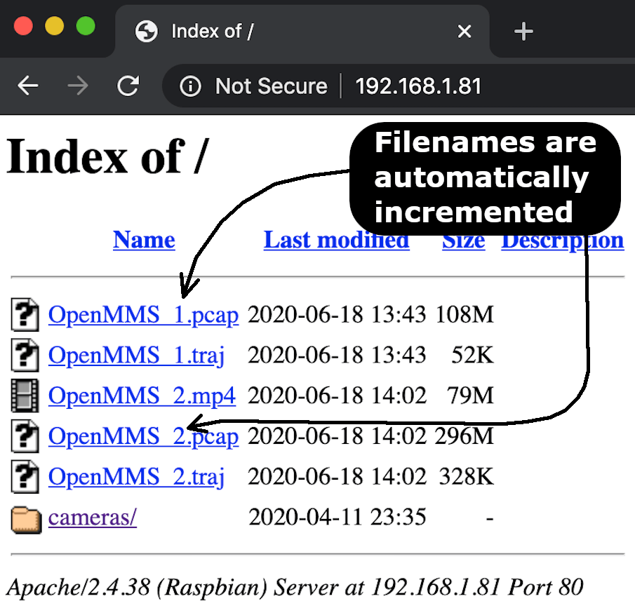
Fig 13.10-1. RPi WebUI Main Page
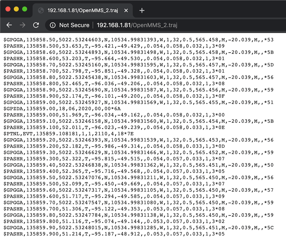
Fig 13.10-2. RPi WebUI View of .TRAJ file
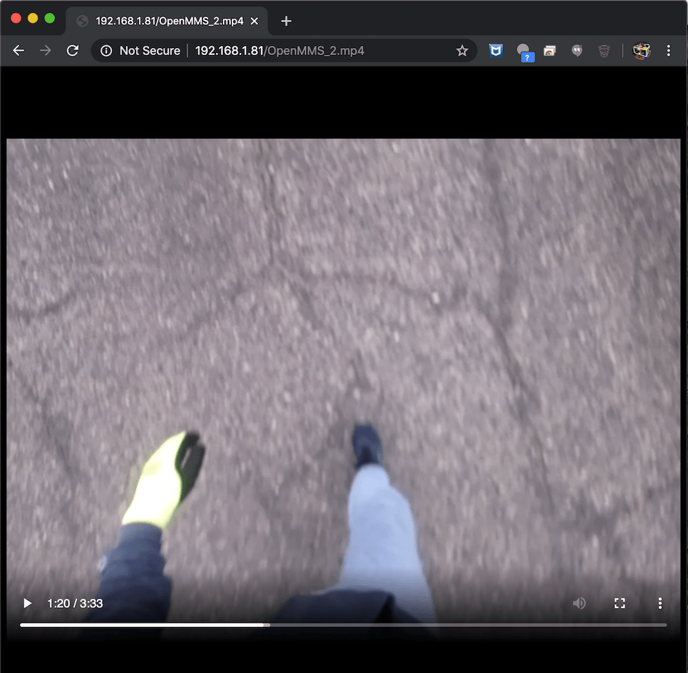
Fig 13.10-3. RPi WebUI View of .MP4 file
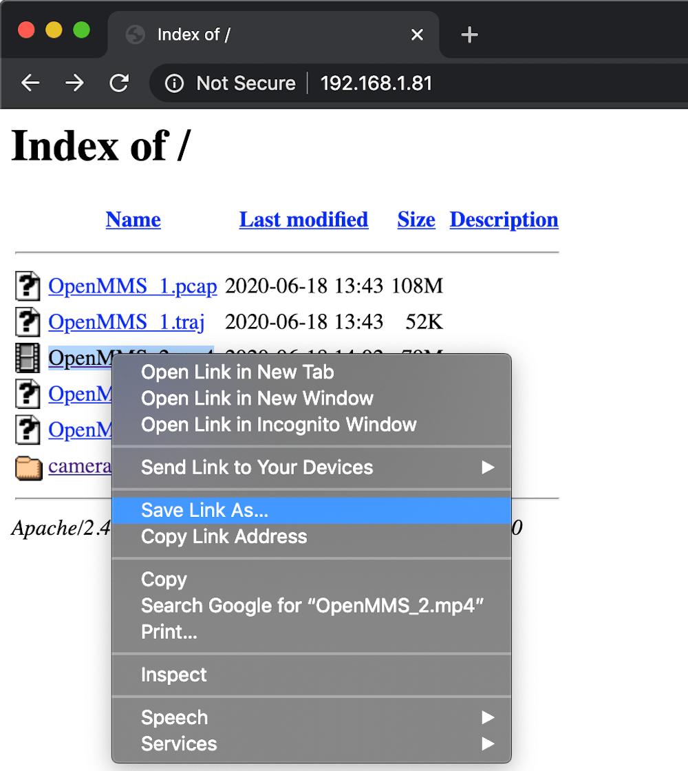
Fig 13.10-4. Right-click to Download files
As mentioned, the RPi’s WebUI also provides the user with access to some important camera settings. Within the main page, click the cameras directory, and a new WebUI page will be displayed. Within the OpenMMS Cameras Configuration page, the user should first click on the Query button to see the current camera settings. IMPORTANT NOTE: the setting options on this page DO NOT display the currently saved values. To change either the Sony A6000 Trigger Interval setting or the Raspberry Pi Camera (Nadir Video) setting, the user first needs to select the new value for the respective setting and then click on the corresponding Set button. A dialog box will appear confirming the new setting value. Click the web browser’s Back Arrow button to return to the WebUI’s main page.
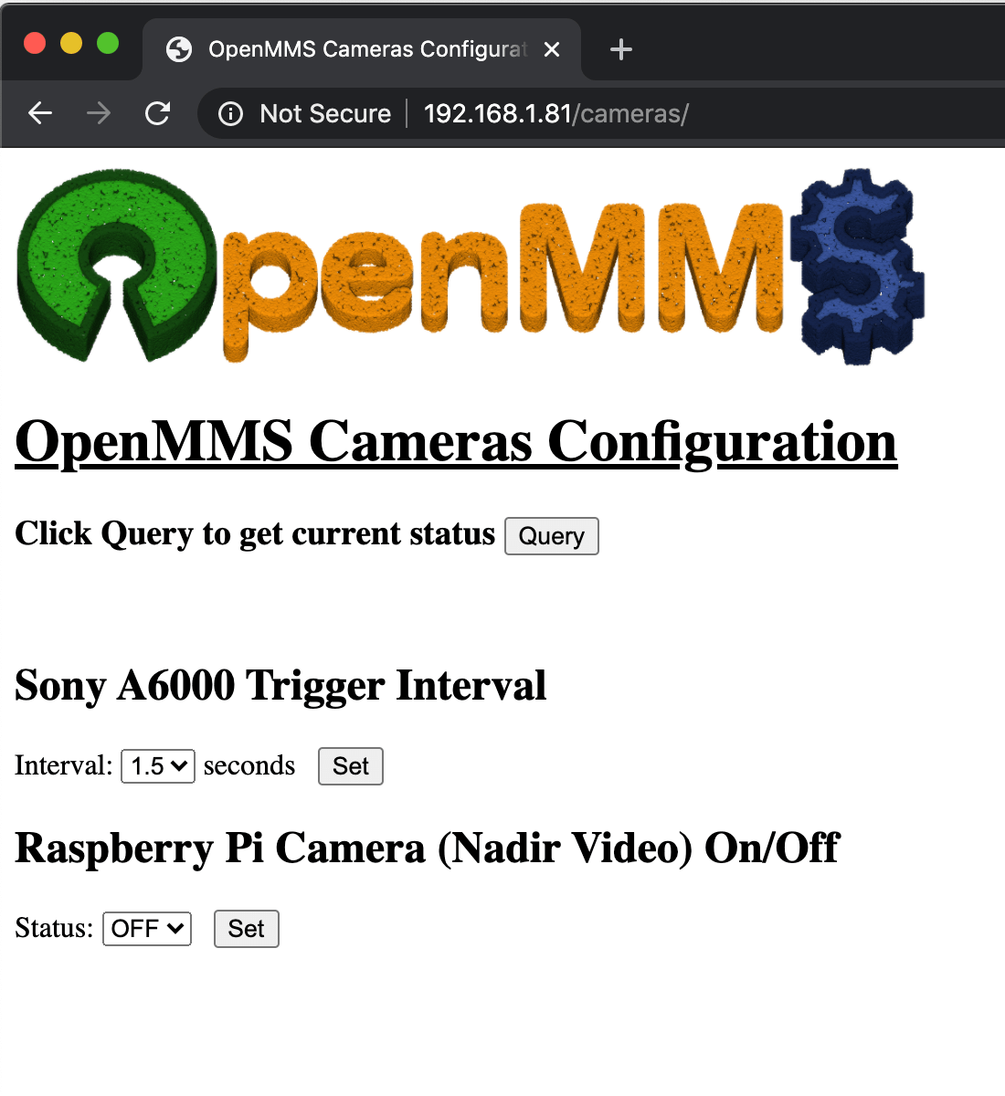
Fig 13.10-5. Cameras Configuration Page
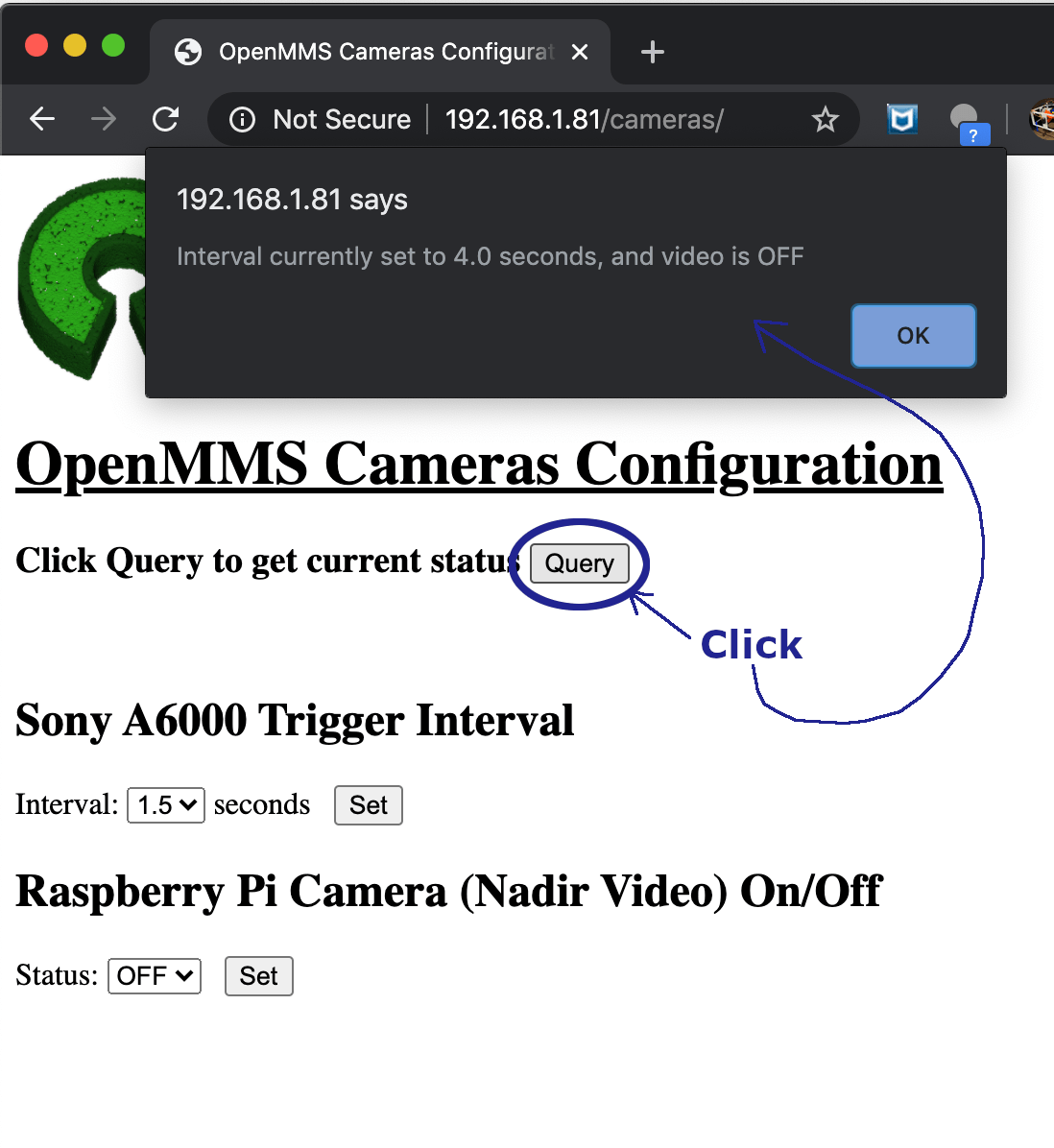
Fig 13.10-6. Query to see the current values
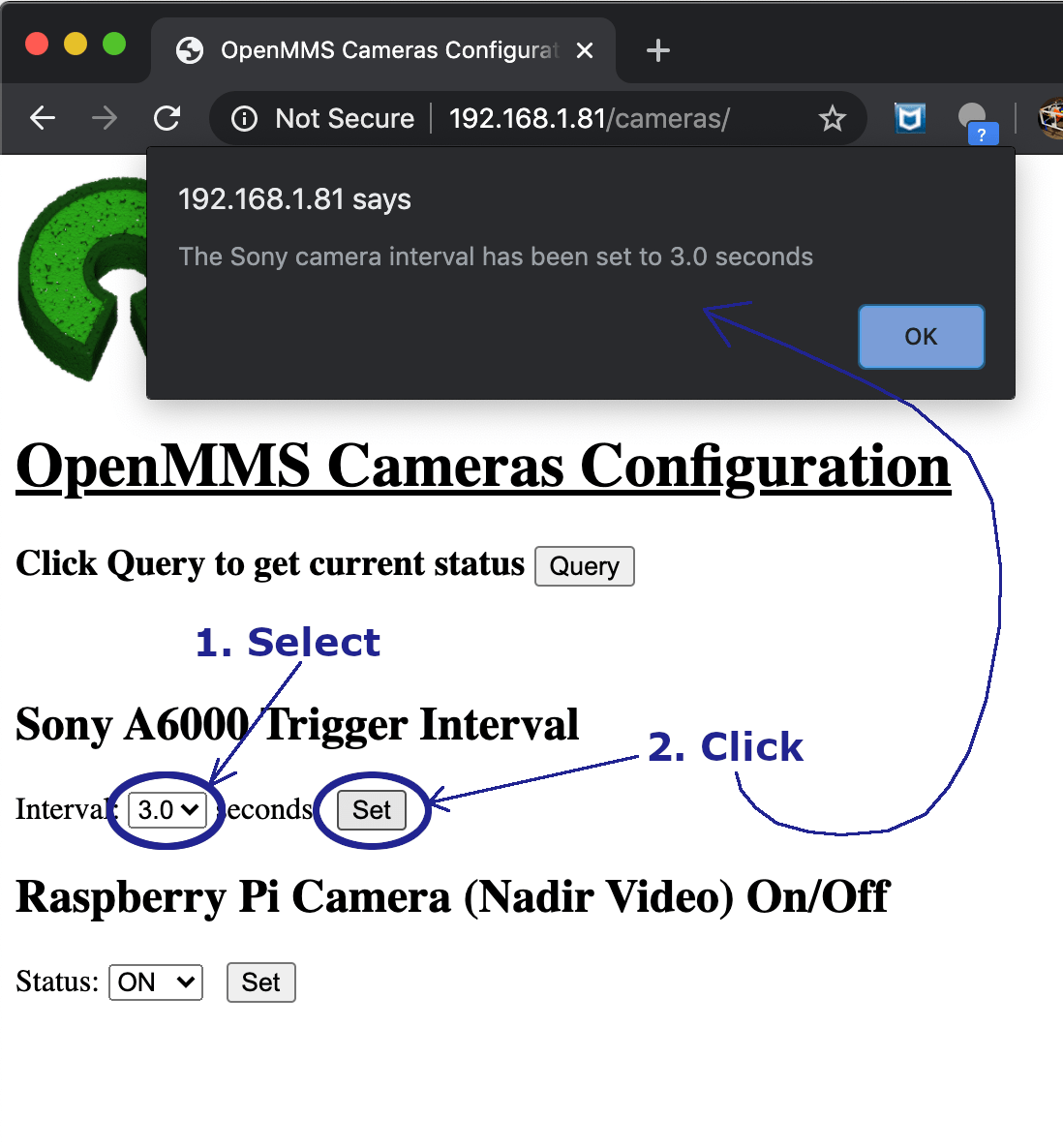
Fig 13.10-7. Update the Interval setting
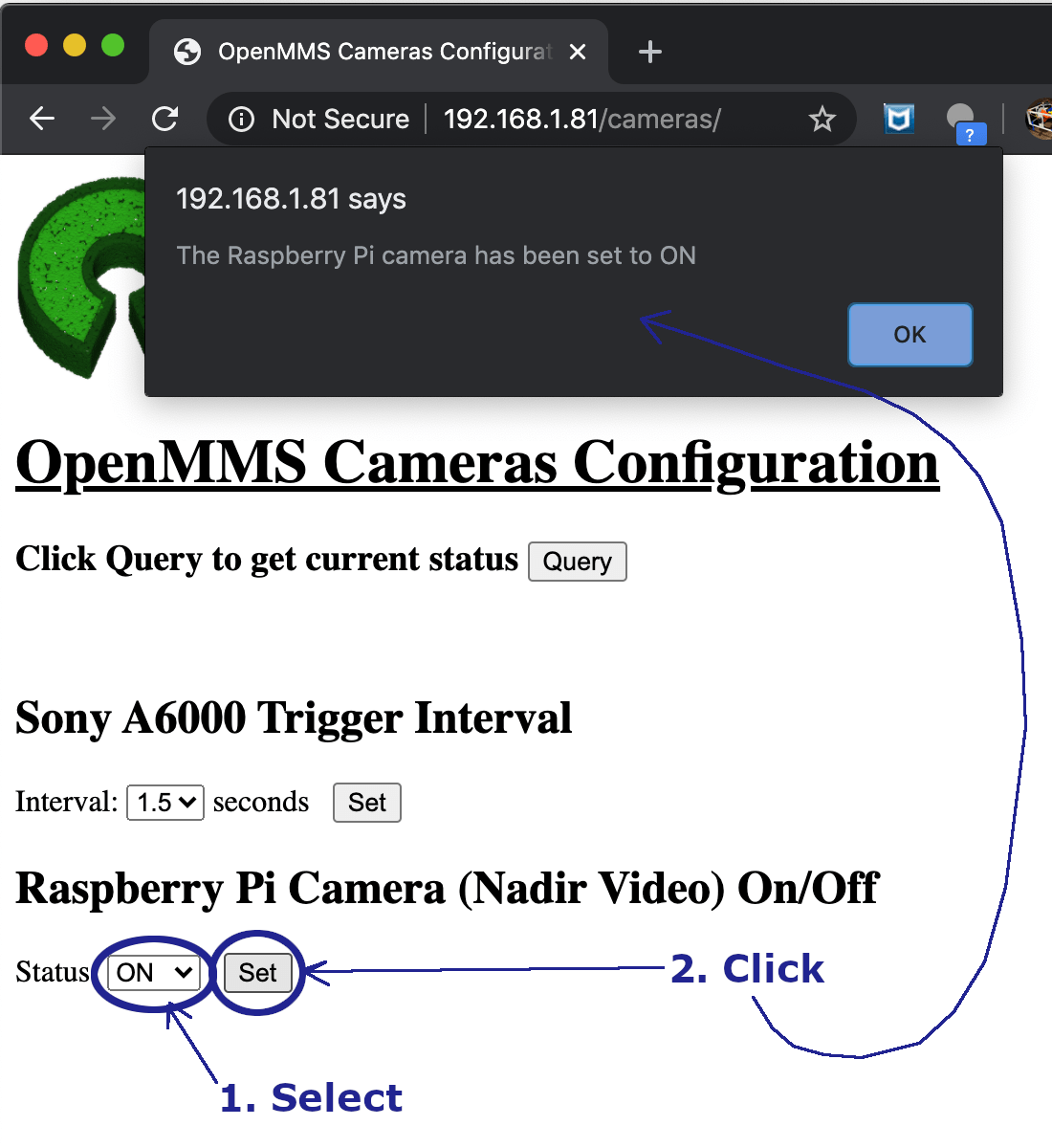
Fig 13.10-8. Update the Video setting
Caution
For the true Open-Sourcians reading this, the Raspberry Pi computer can be directly accessed via SSH using the username:password of openmms:$mmnep0 (where the last character in the password is the number zero). HOWEVER, DO NOT CHANGE THE USERNAME OR PASSWORD, OR THE REAL-TIME CONTROLLER CODE WILL BREAK AND THE SENSOR WILL NOT OPERATE PROPERLY!
13.11. Access the Applanix APX-18
Warning
The reader’s computer needs to be physically connected to the OpenMMS sensor using an ethernet cable and assigned an appropriate static IP address and subnet mask to successfully connect to the APX-18. An IP address of 192.168.1.23 and a subnet mask of 255.255.255.0 are recommended.
As discussed in section 8.6, the Applanix APX-18 sensor provides the user with a Web-based User Interface (WebUI) to access the sensor’s settings and the data files stored within its internal 8 GB of data storage. After completing a data collection campaign, the user needs to access the WebUI and download the necessary .T04 data file.
To connect to the APX-18’s WebUI, open a web browser on the connected computer and enter the address of 192.168.1.200 into the URL textbox and press enter. The login information is admin:password (username:password). Then in the left-hand column, click on Data Logging, then on Data Files, and then on the Internal directory (if shown). The date corresponds to the start time of the data logging in GPS time. The filename for a .T04 file (as configured for the OpenMMS sensor) starts with the serial number for the APX-18 sensor, followed by the 4 digit year, the 2 digit month, the 2 digit day, y the 2 digit GPS hour, and lastly the 2 digit GPS minute for the start time of the data file. See the figure below for an example. To download a single .T04 file, all users have to do is click on the .T04 filename within the list. Alternatively, multiple .T04 files can be downloaded together by clicking the checkboxes on the right side of each file, and then click on the Download Selected Files option.
Tip
It is recommended to record the GPS/UTC time when the NAV pushbutton is latched during a data collection campaign, so this timestamp can be used to ensure the correct .T04 file is downloaded.
If it appears that the .T04 file for the most recent data collection campaign is missing from the WebUI list, it is recommended to power off the APX-18 (unlatch the NAV pushbutton), wait for ~ 5 sec. and then power it up again. A data logging file is only closed, and then available within the data files list, after the APX-18 has been powered off.
If the WebUI repeatedly fails to be displayed within a web browser, it is recommended to completely close the web browser application (i.e., all open tabs and/or windows) and restart the web browser. If this still fails, it is recommended to restart both the OpenMMS sensor and the connected computer, and check the computer’s IP address settings.
Additionally, the calibration status of the APX-18’s magnetometer and the number of events recorded within the current data logging session can be viewed within the WebUI. Within the left-hand column, click on Receiver Status, then click on INS Status. The WebUI now displays the screen shown in the figures below. Make a note of the highlighted areas within the figure, as they indicate the calibration status of the magnetometer and the number of recorded events.
Tip
It is always good to compare the number of camera events recorded by the APX-18 with the number of photos taken by the Sony A6000 camera. In theory, the numbers should always match, but from the author’s experience, it does sometimes happen that the numbers do not match. Within the upcoming OpenMMS Software - Data Processing Workflow section, an image pre-processing procedure is discussed that helps combat this issue if experienced.
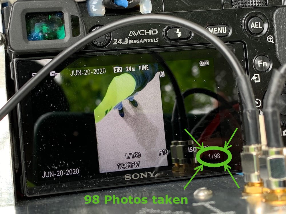
Fig 13.11-5. Seeing how many photos were taken
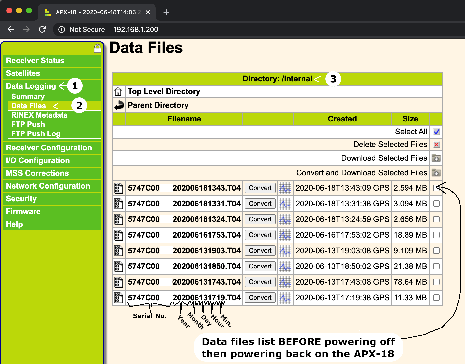
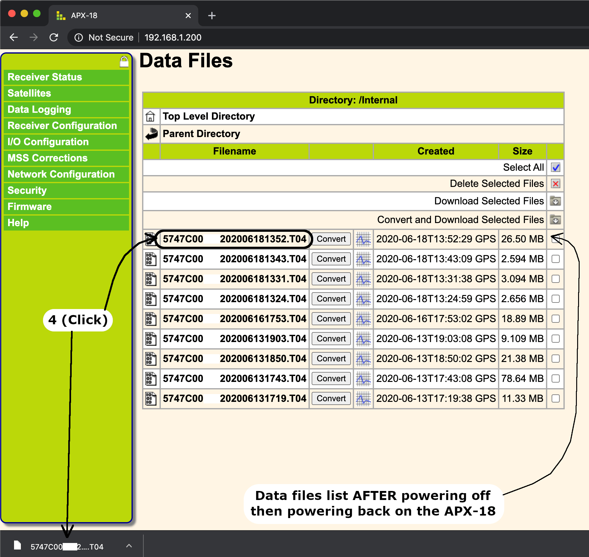
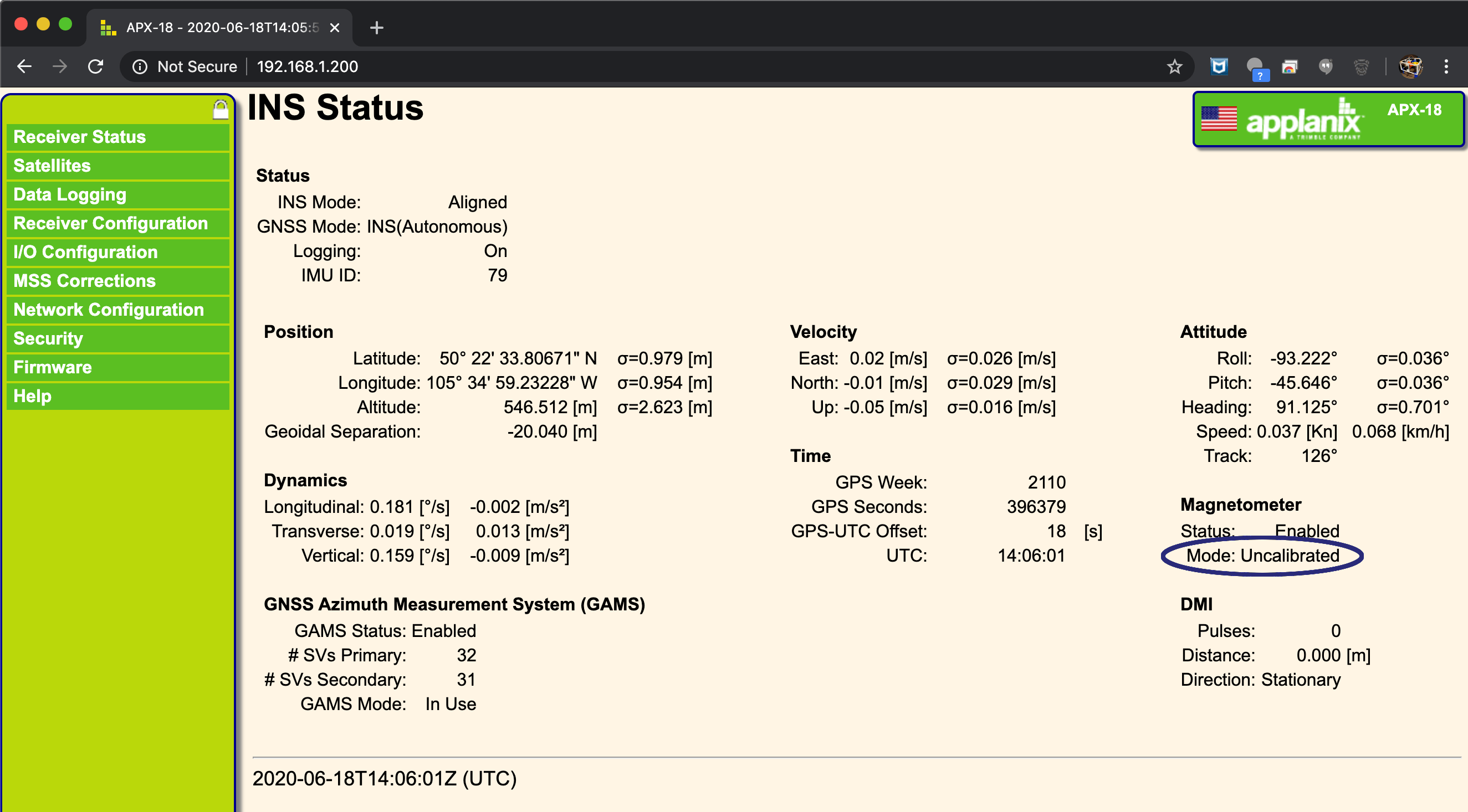
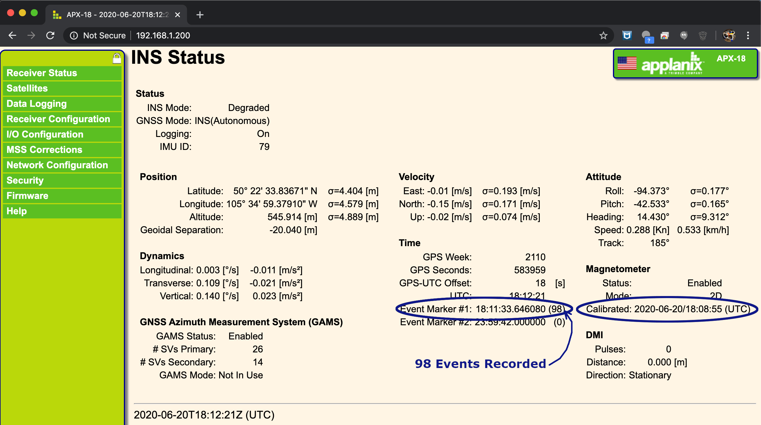
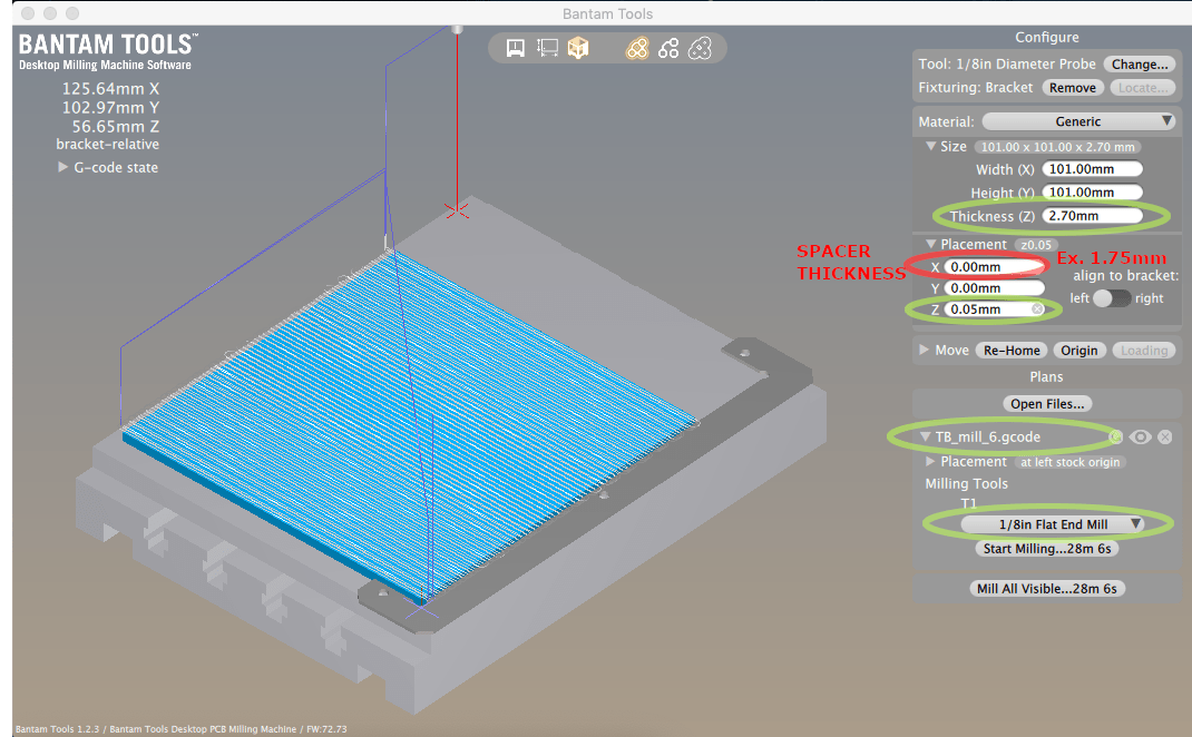
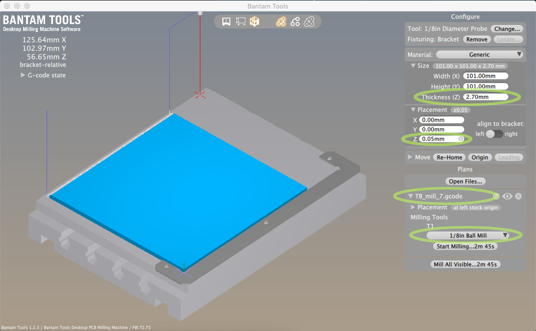
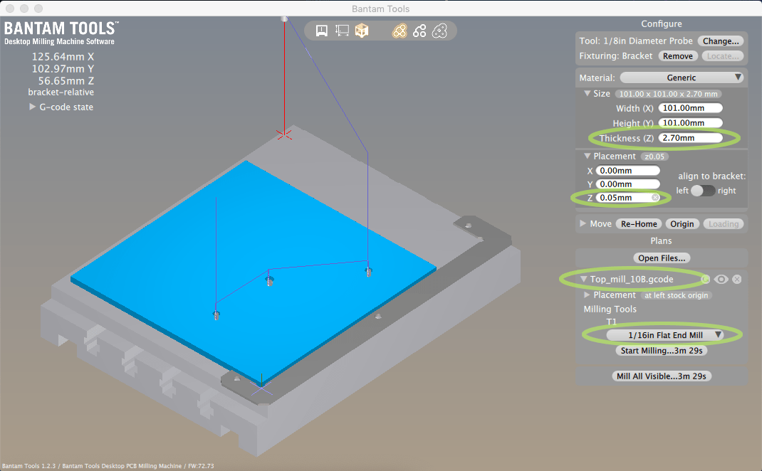
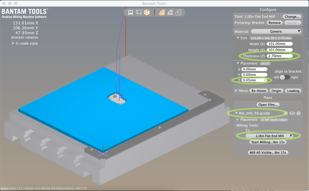
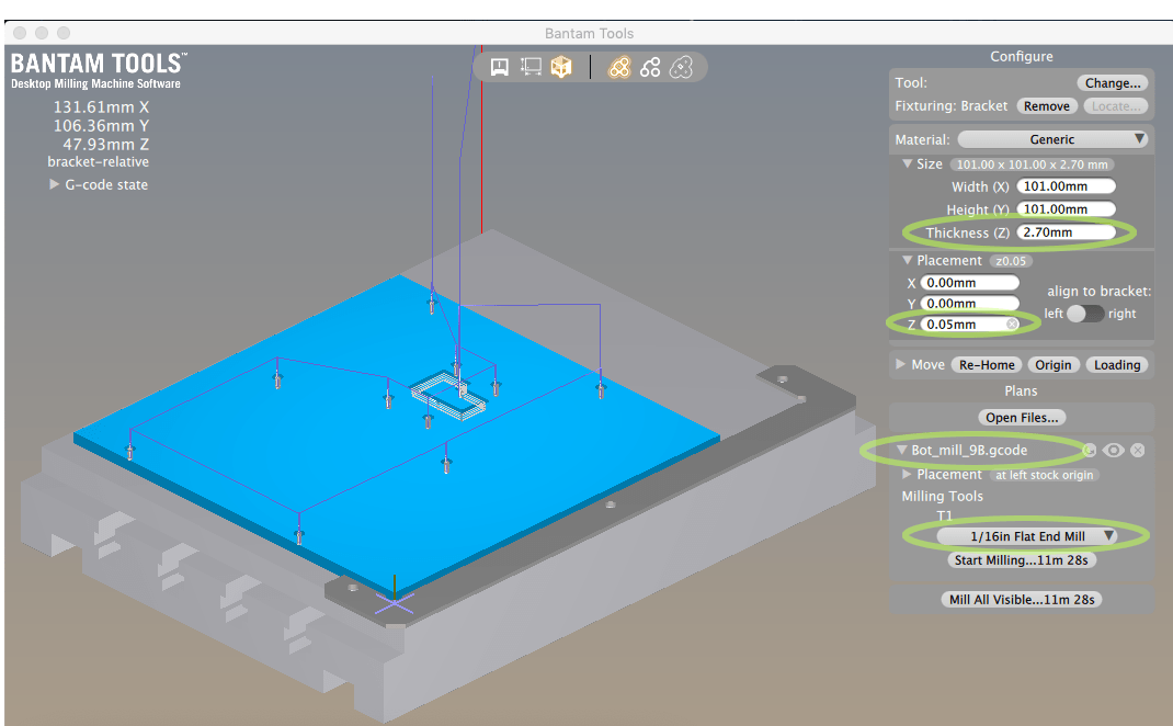
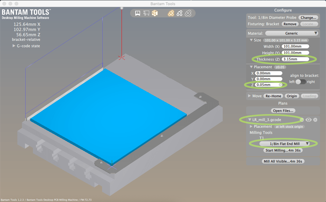
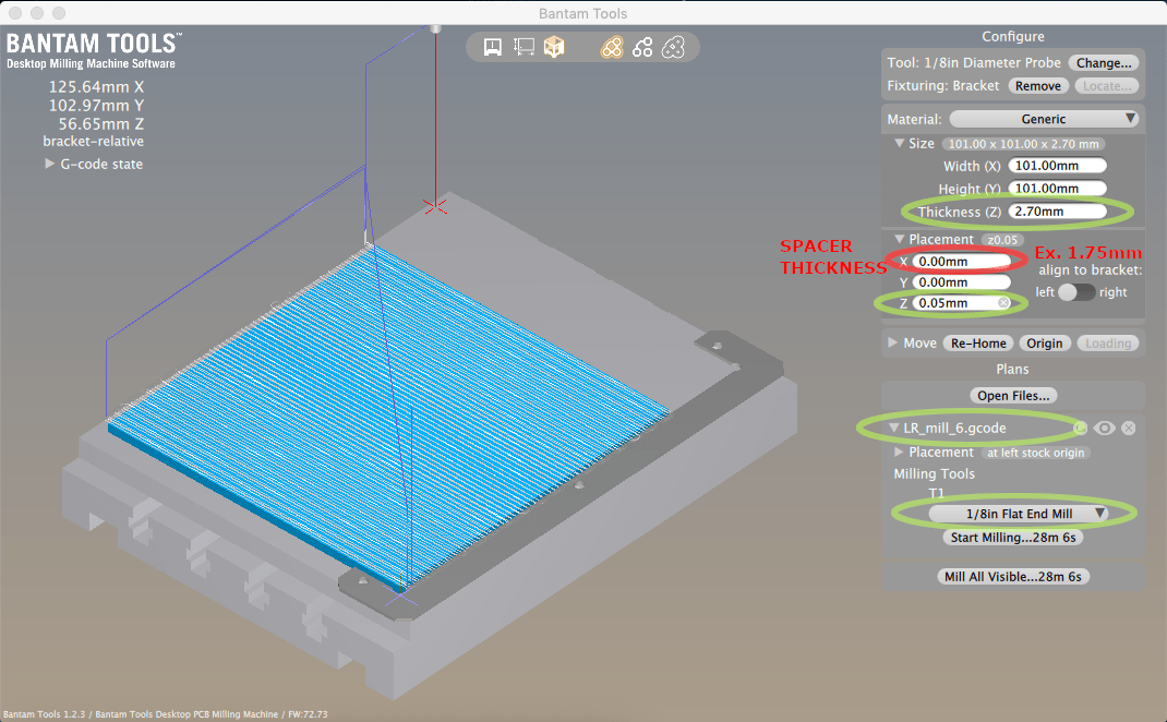
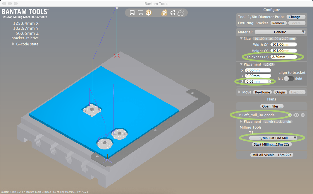
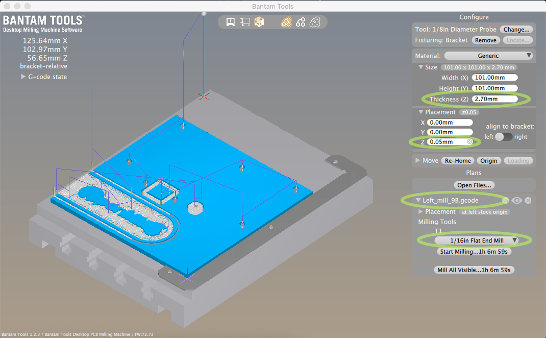
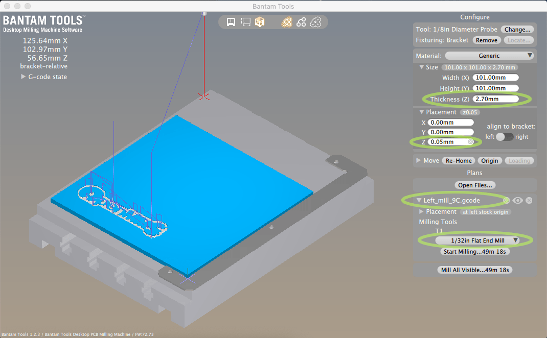
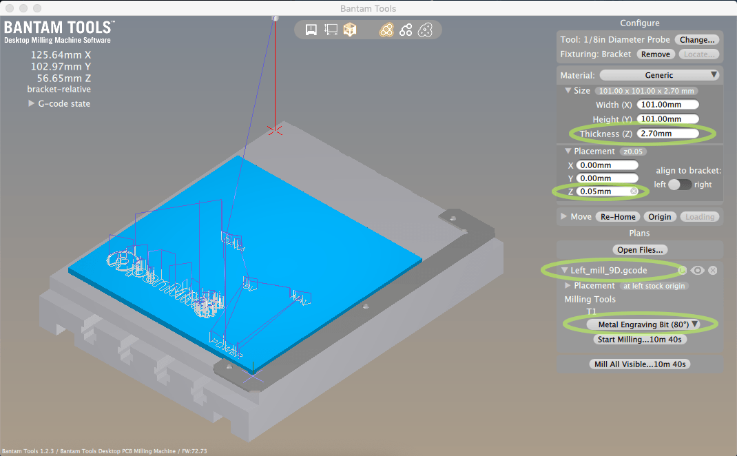
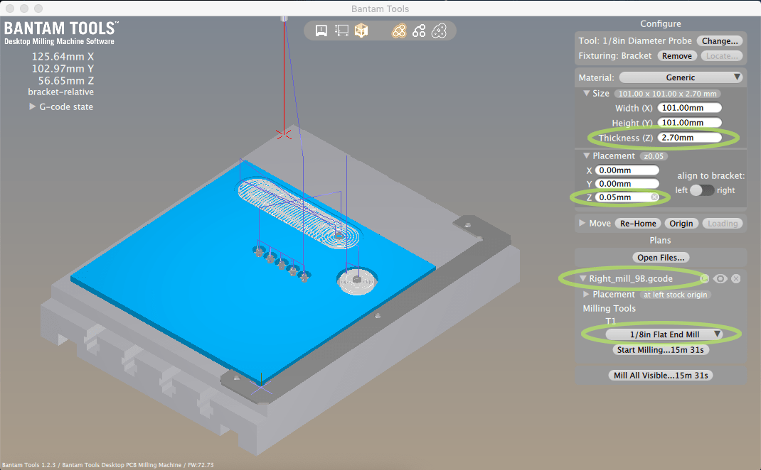
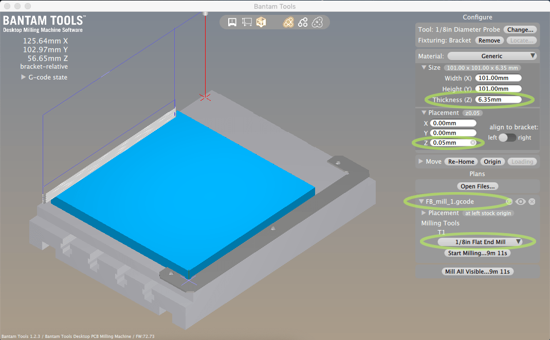
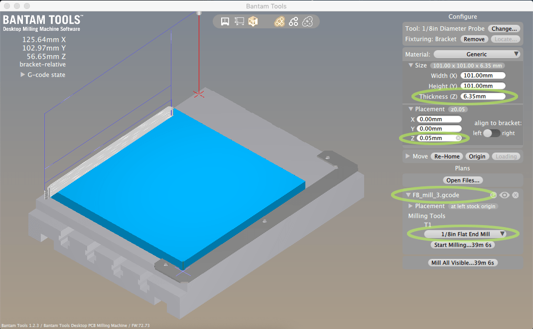
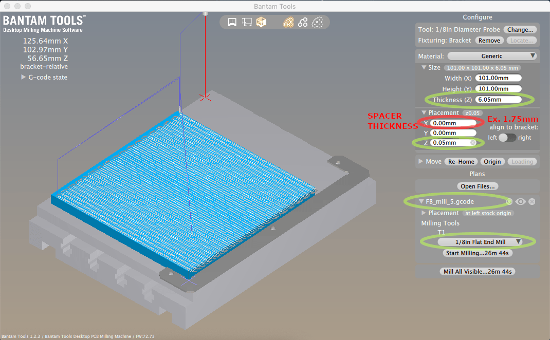
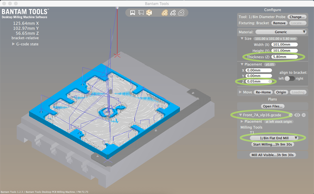
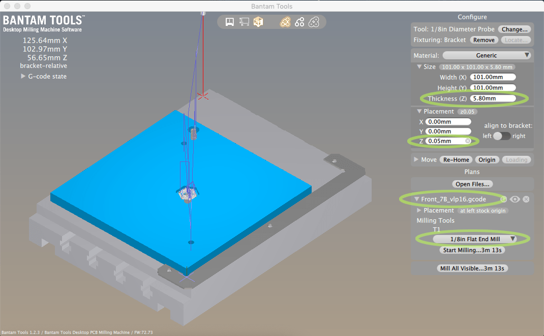
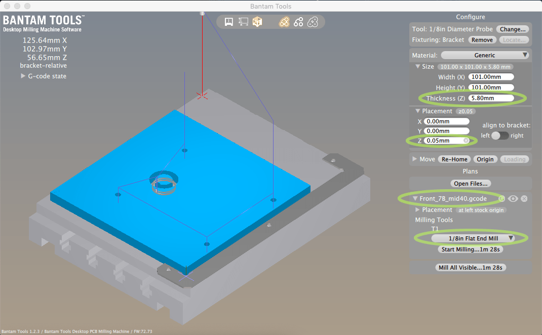
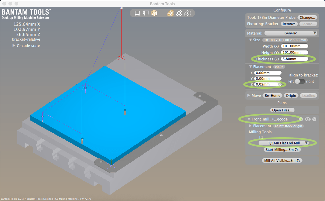
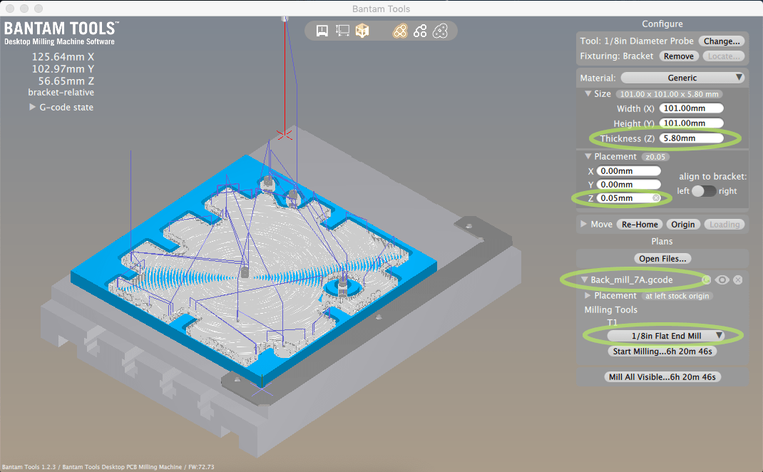
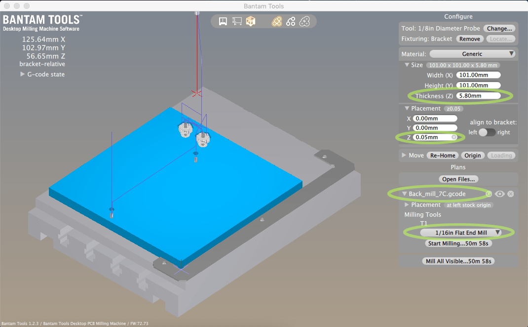
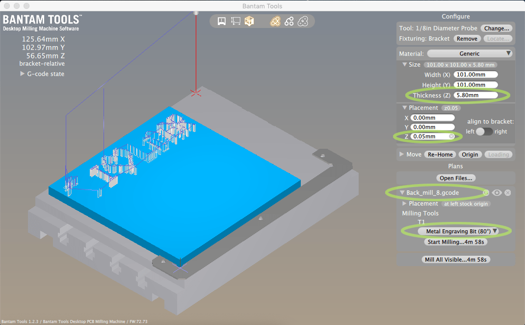
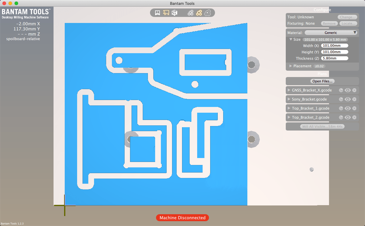
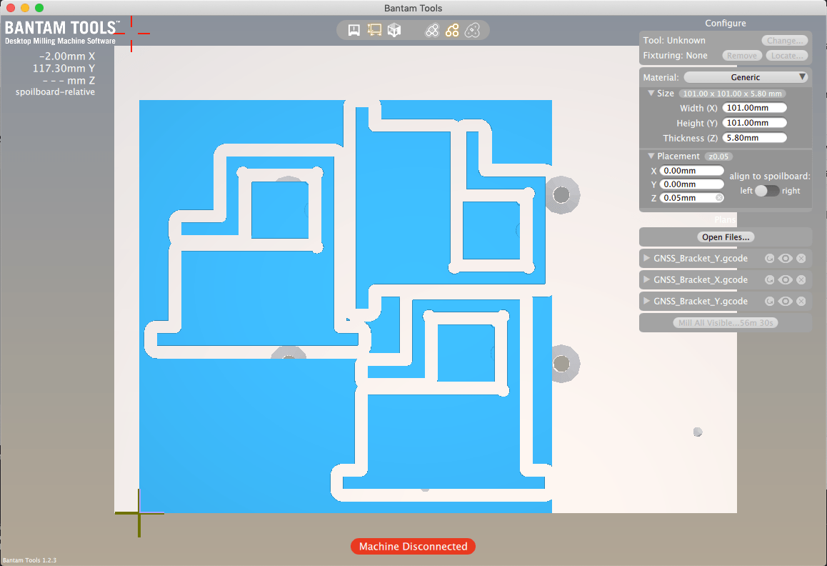
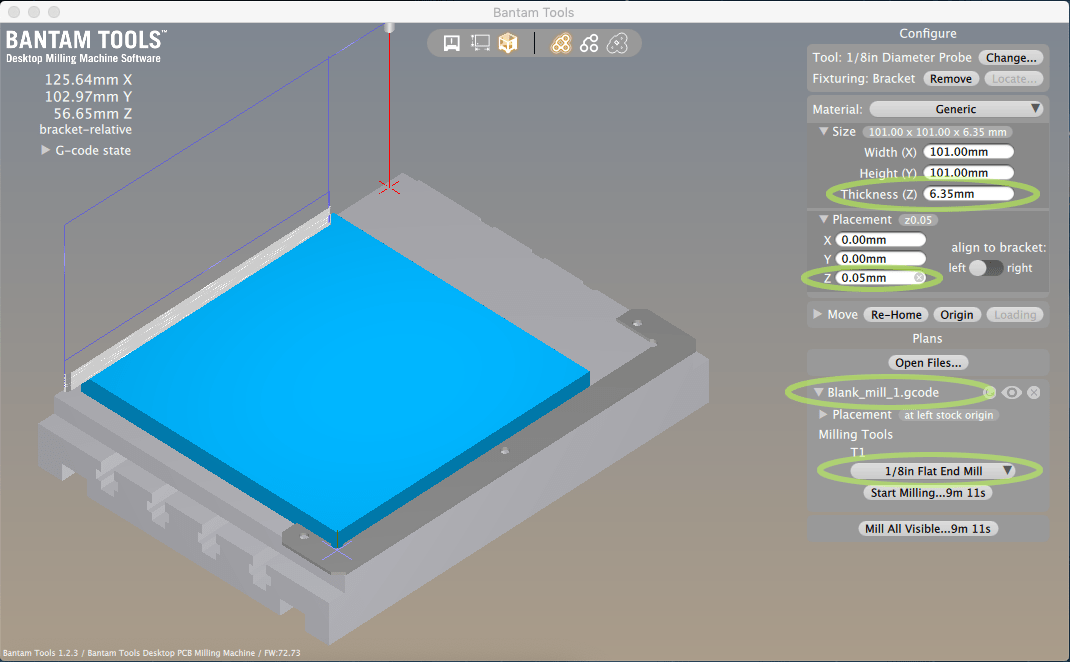
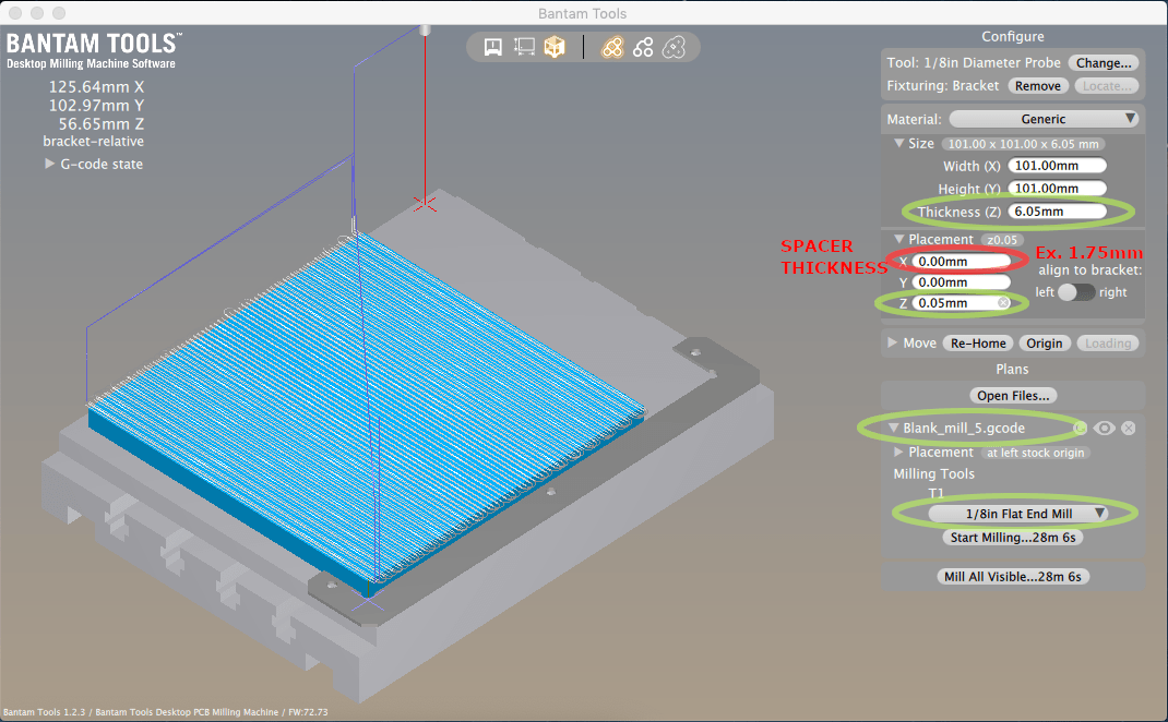
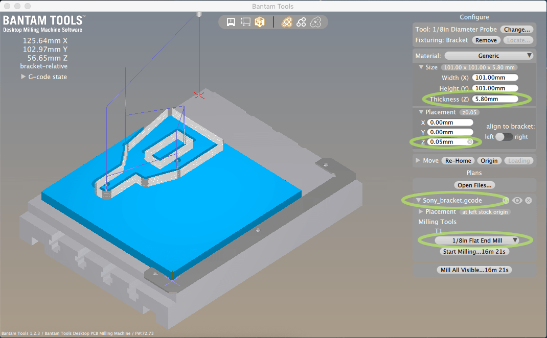
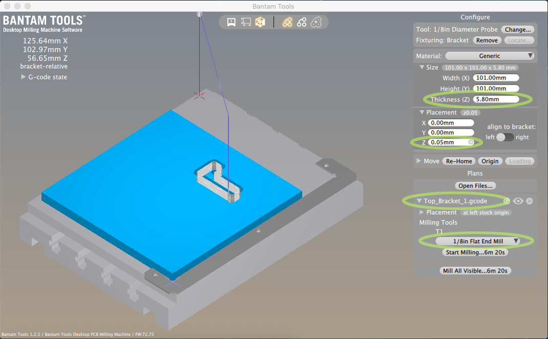
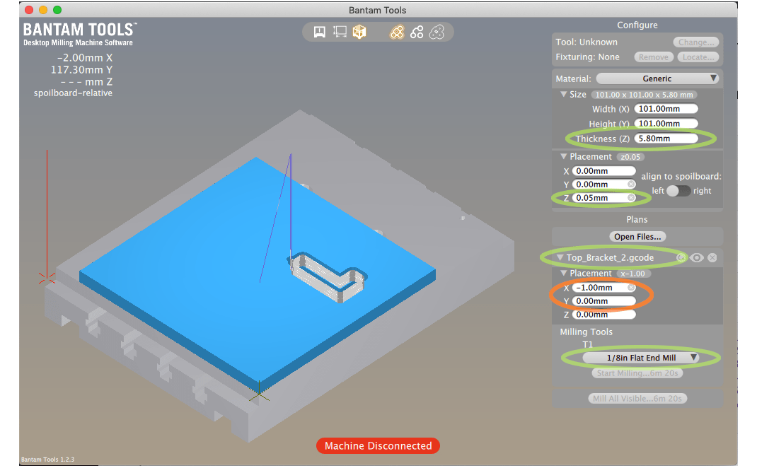
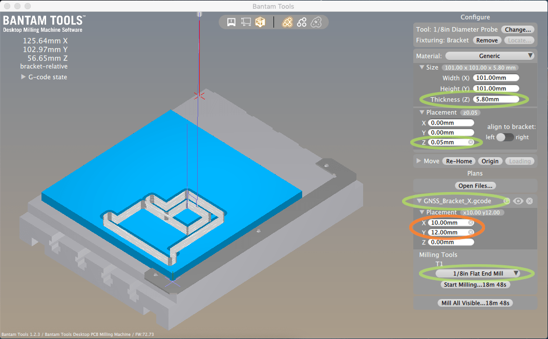
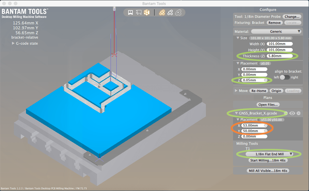
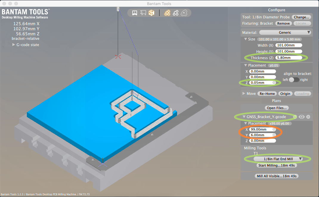
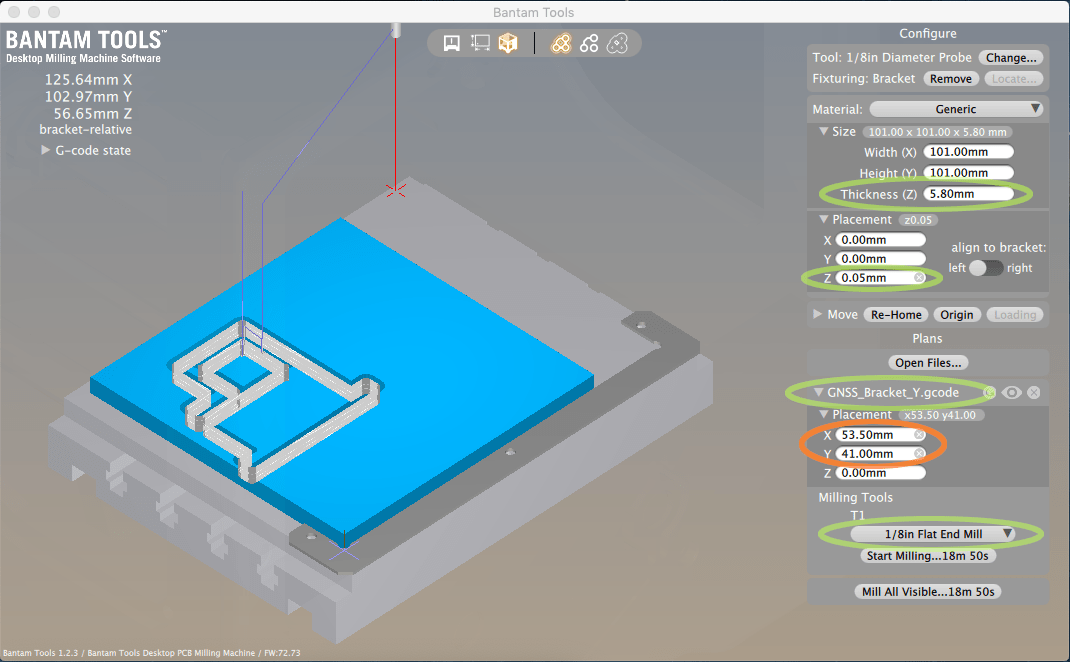
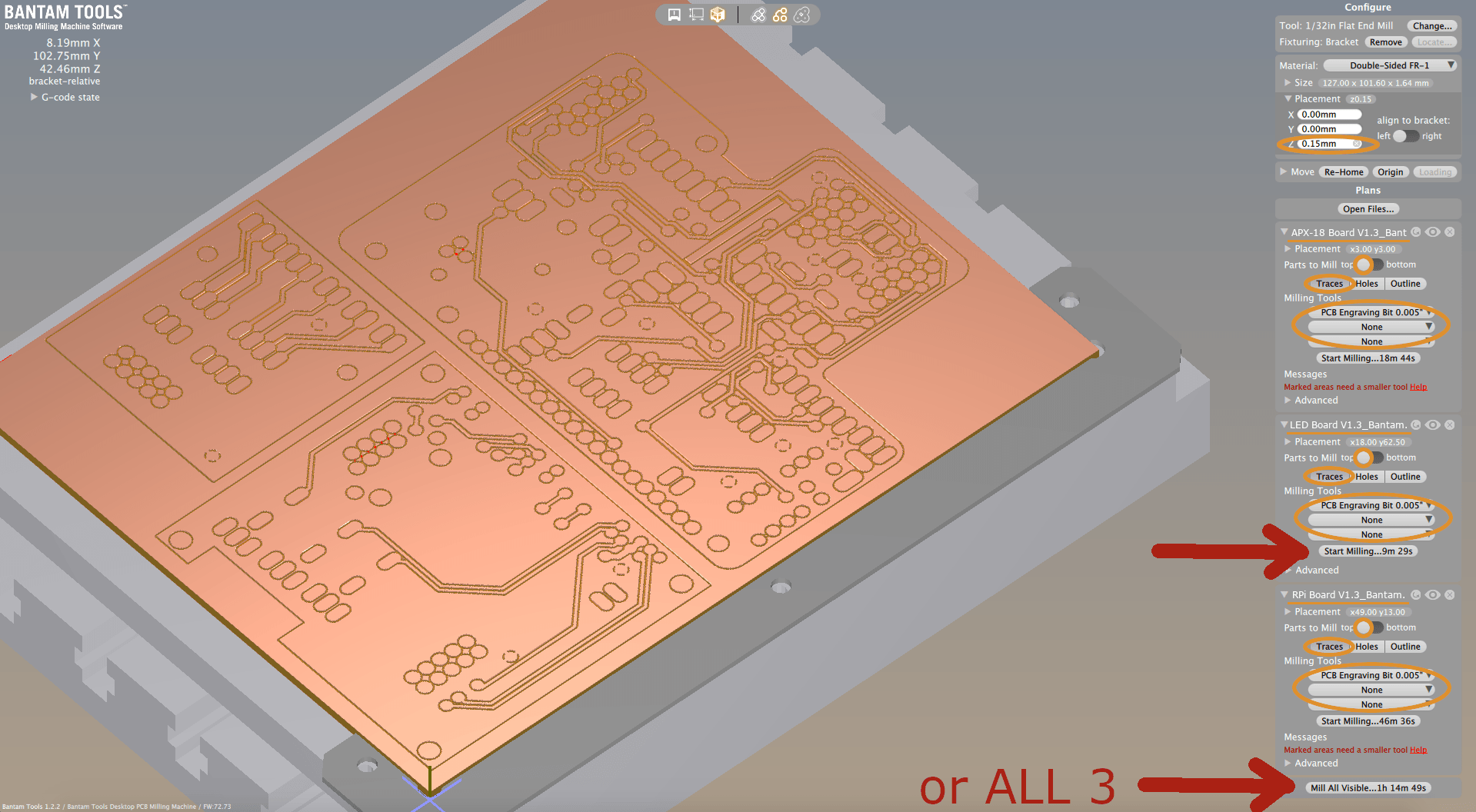
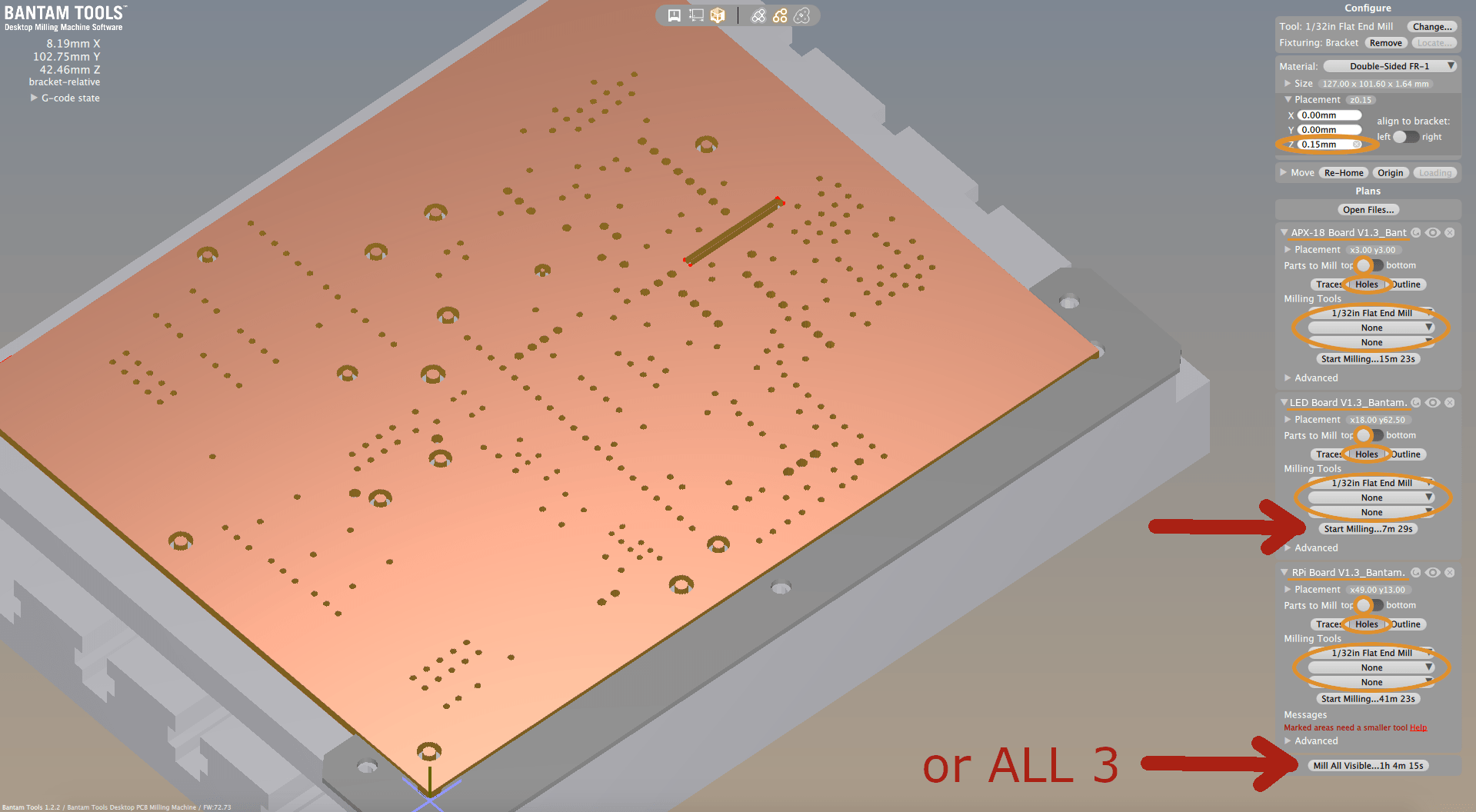
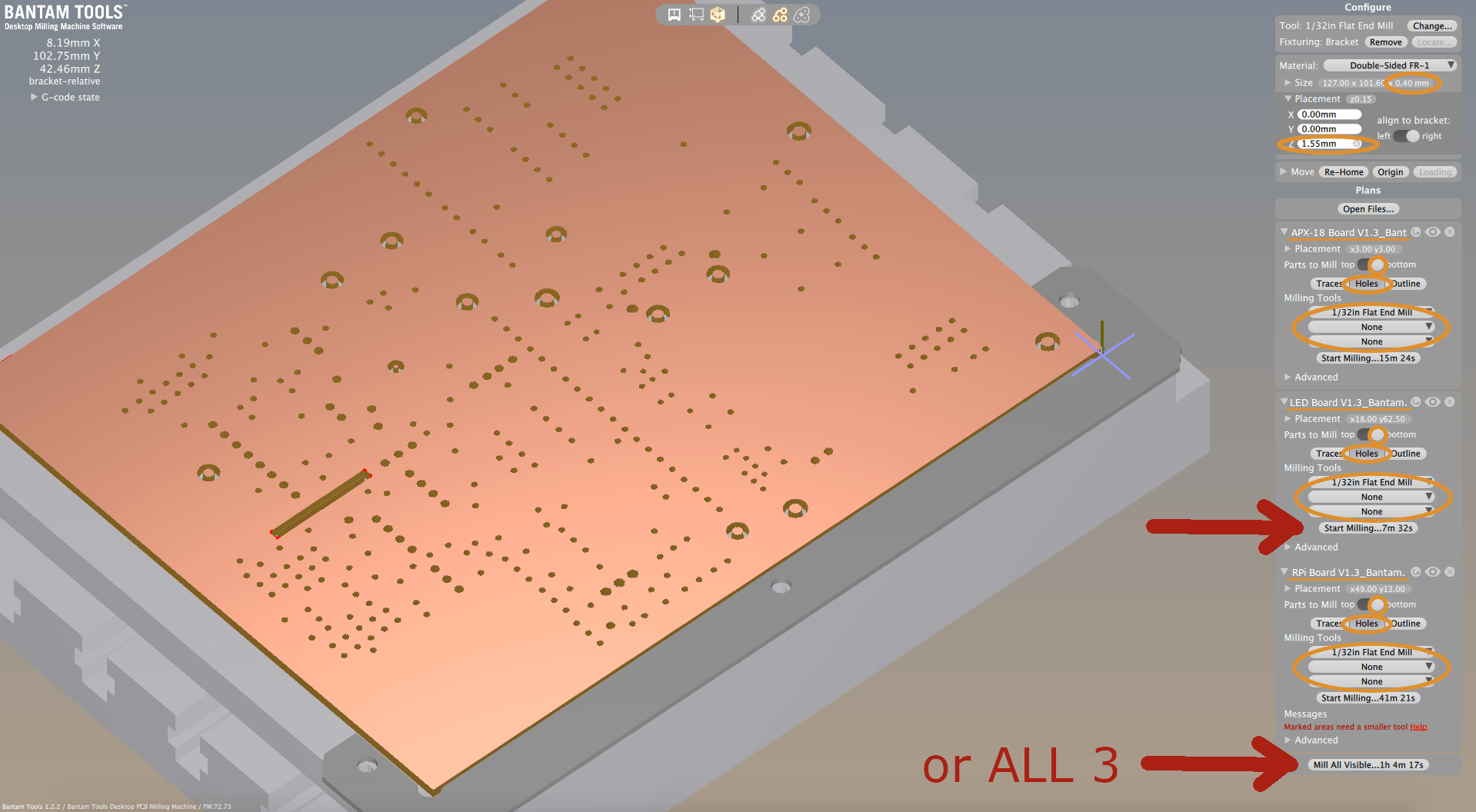
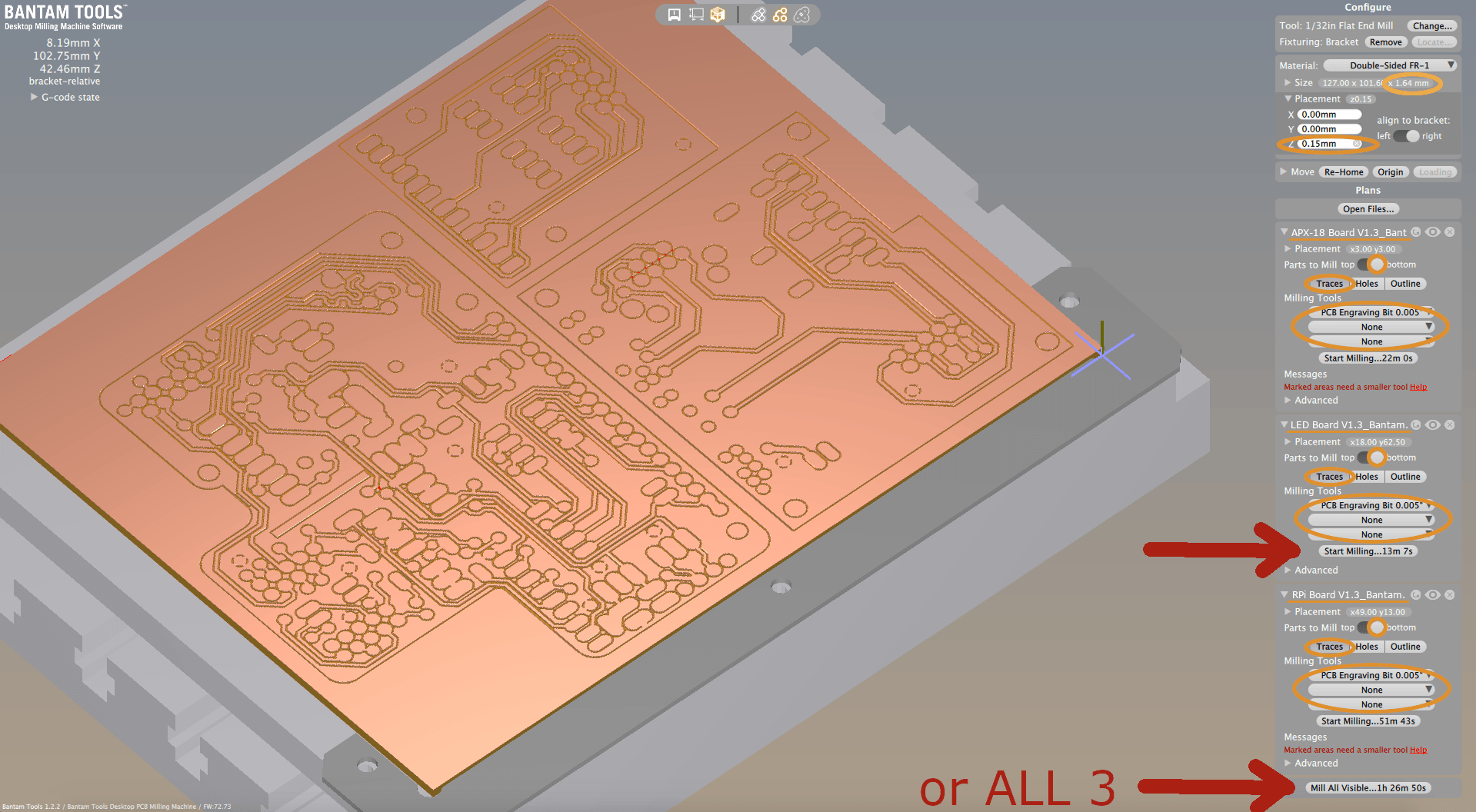
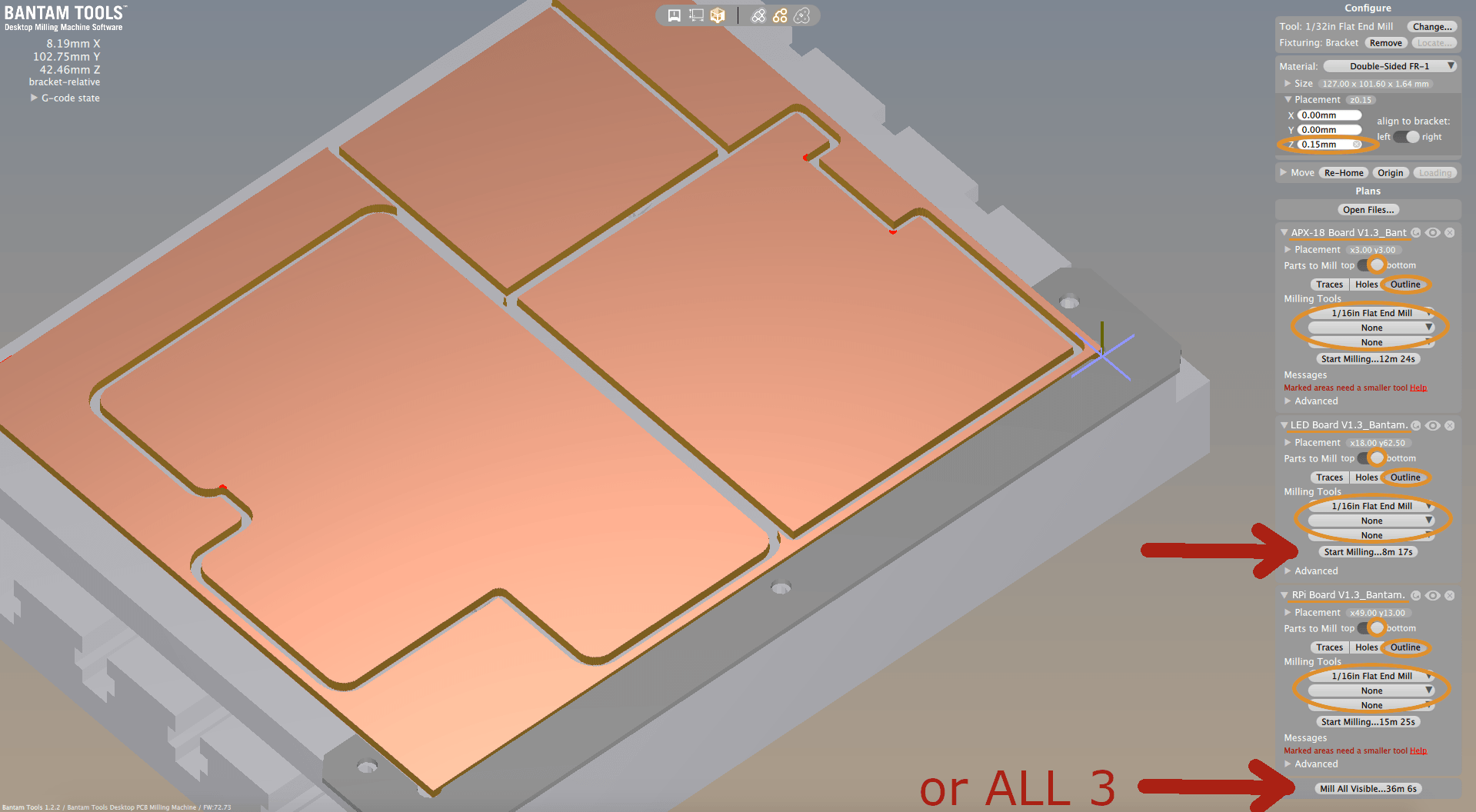
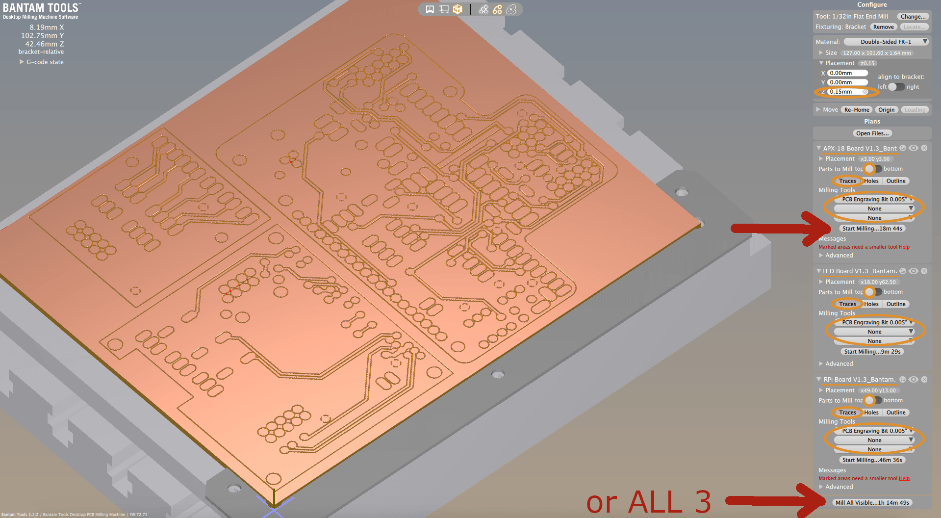
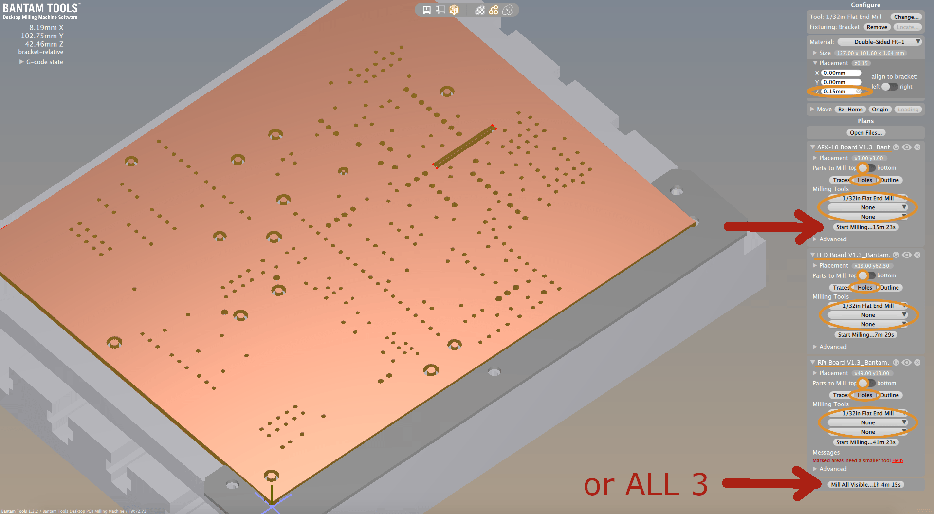
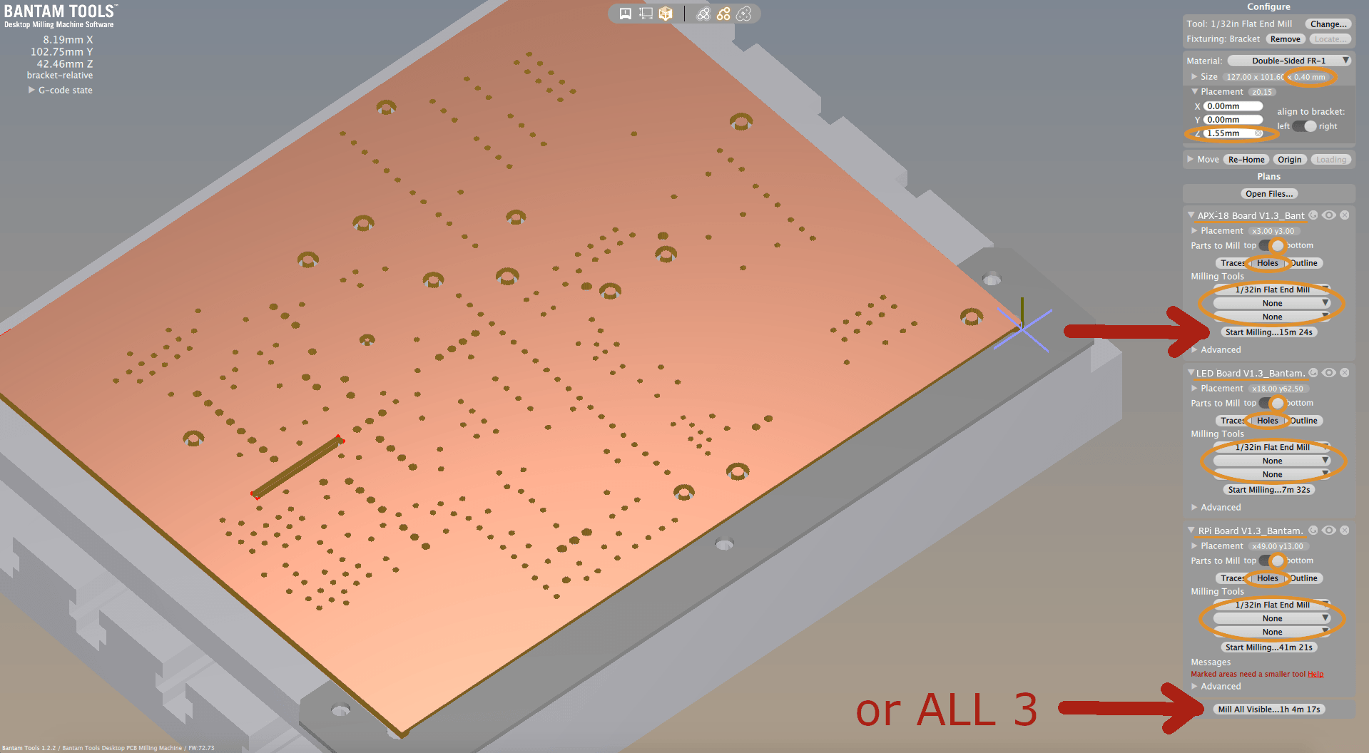
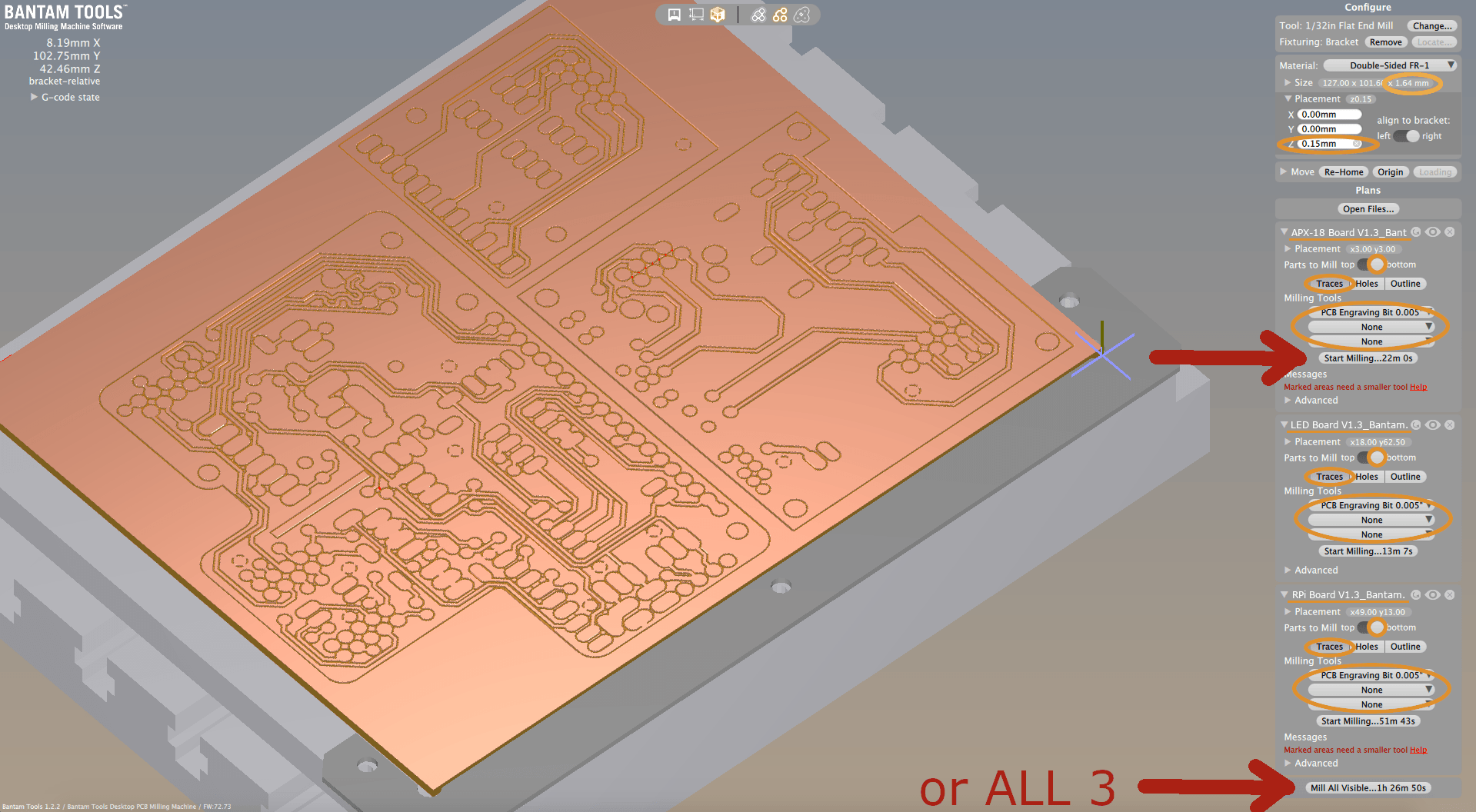
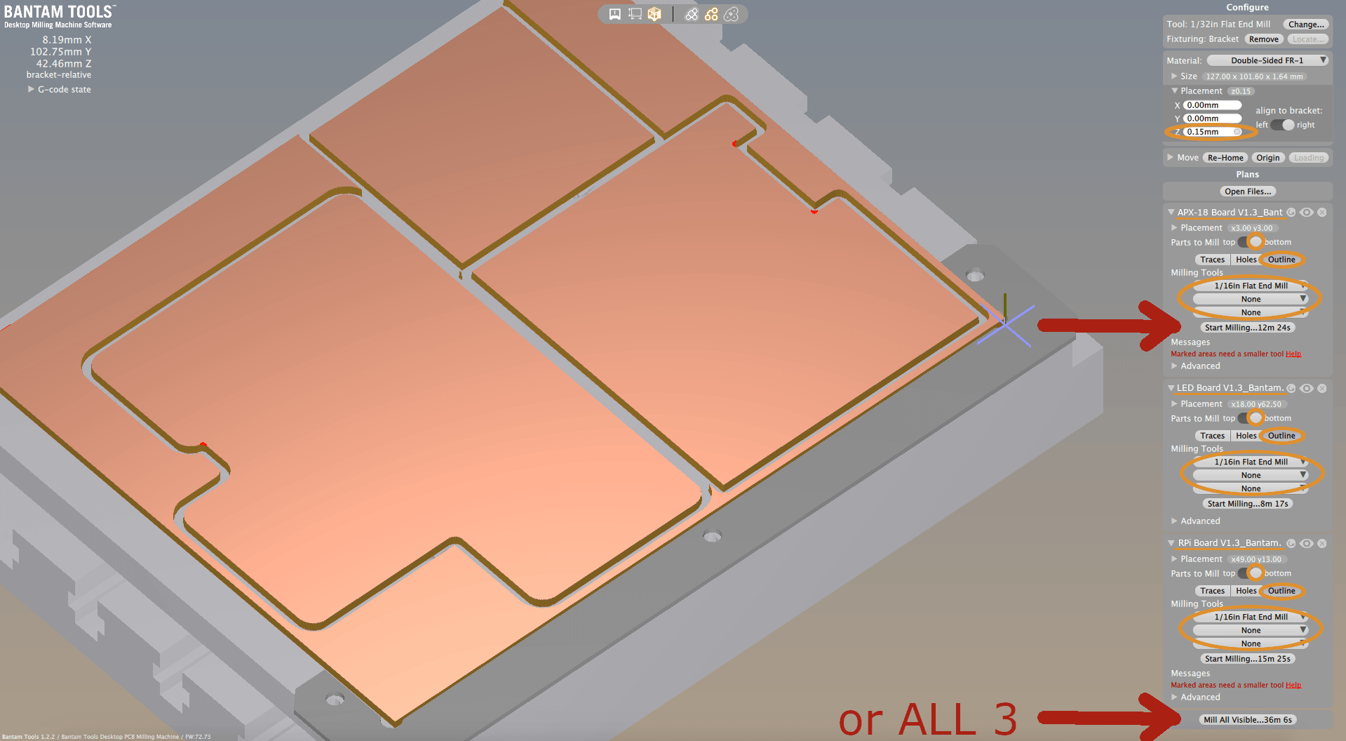
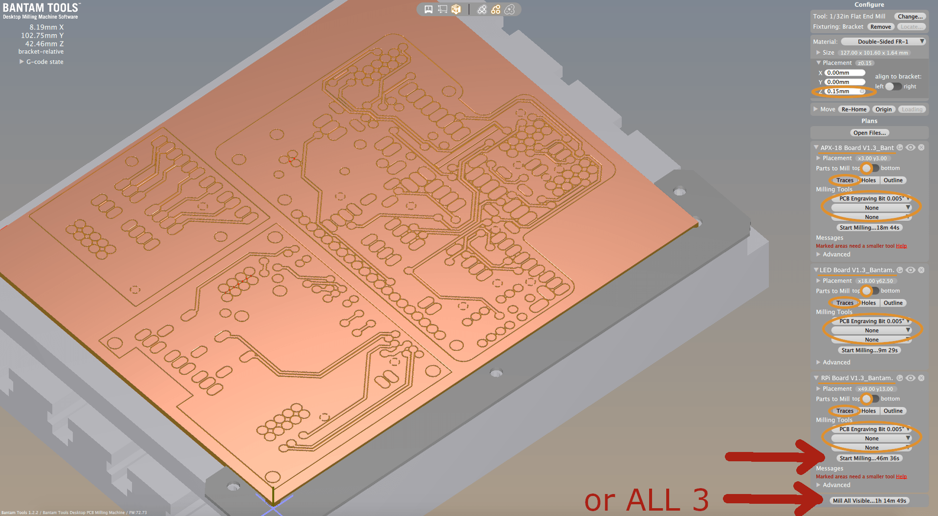
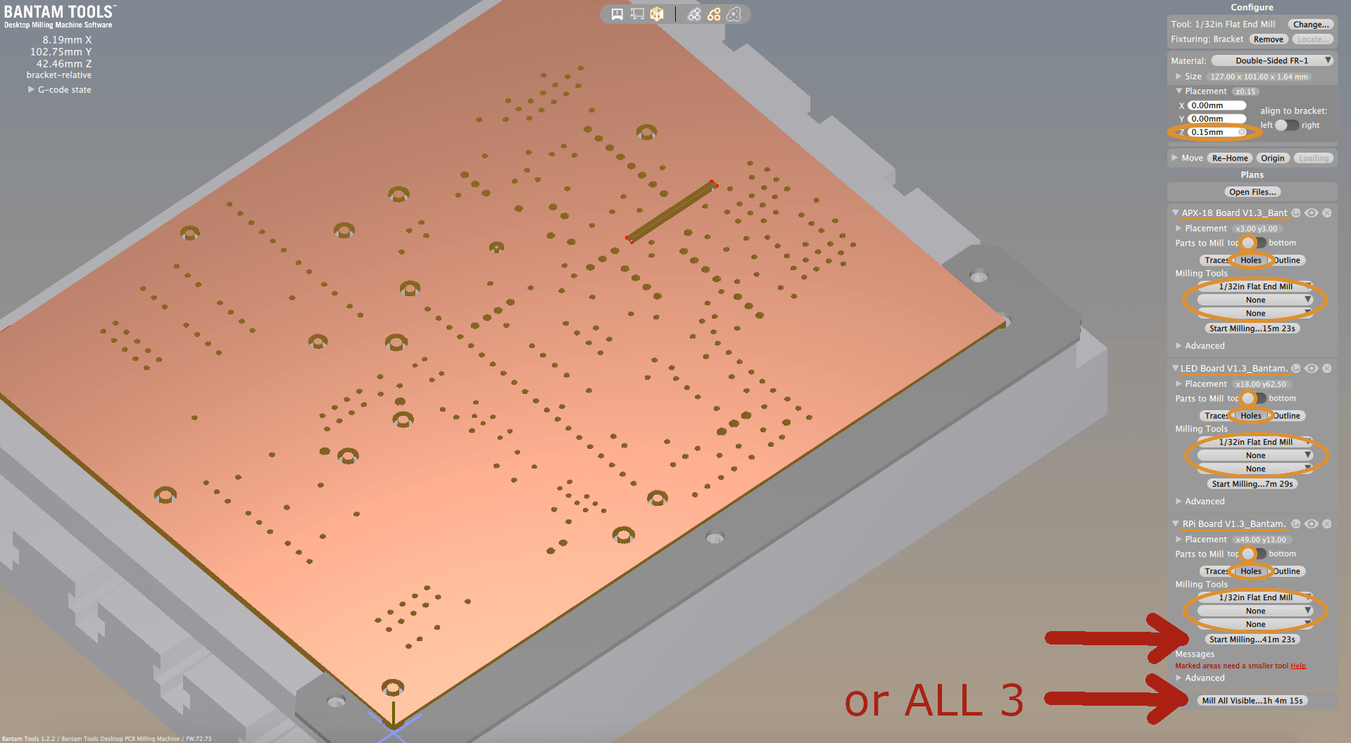
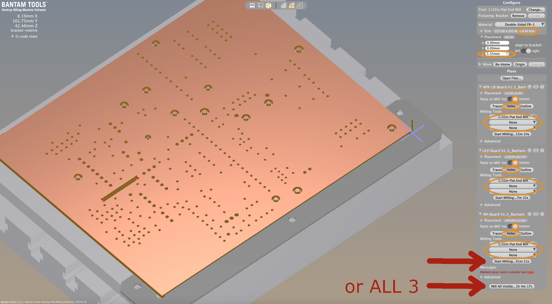
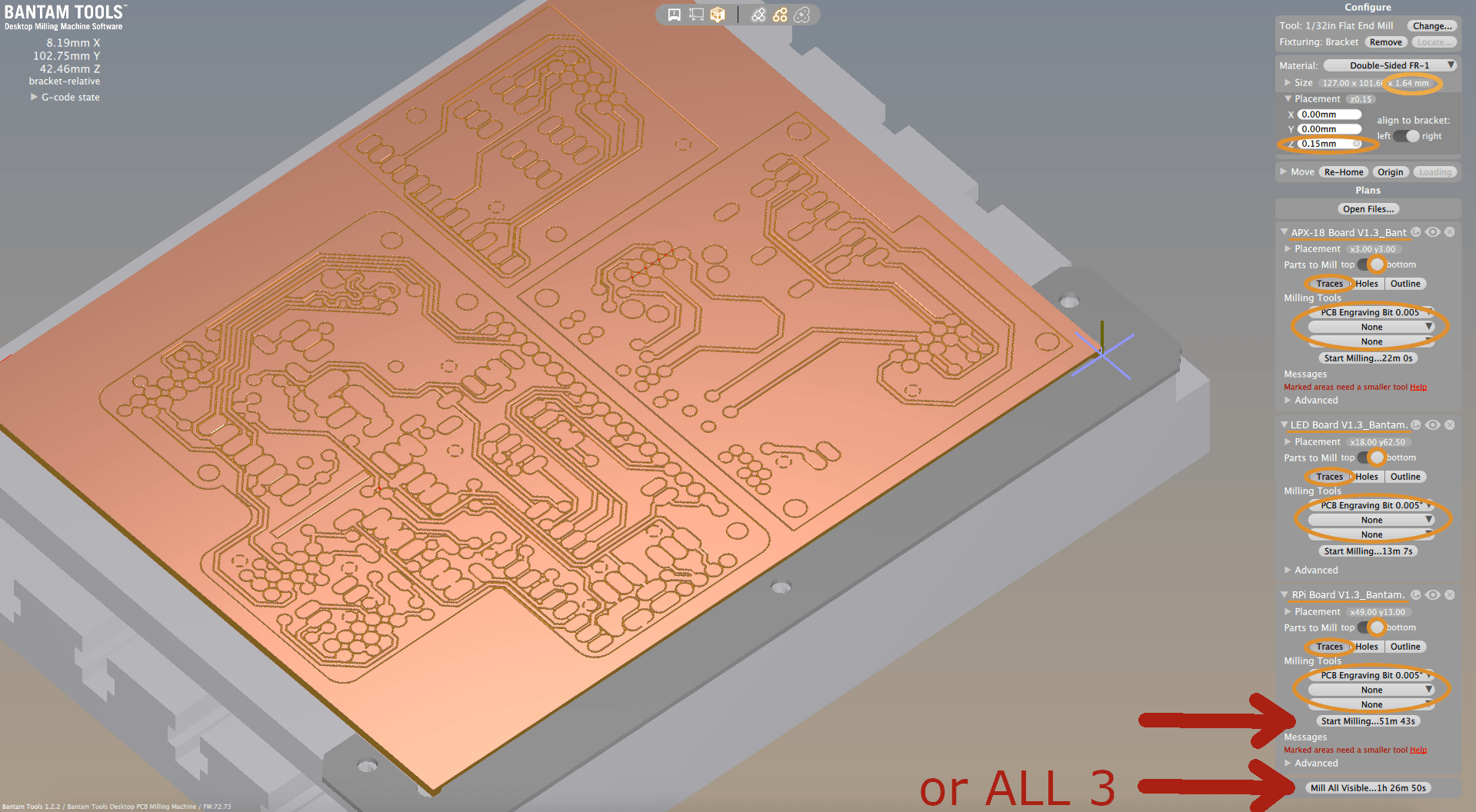
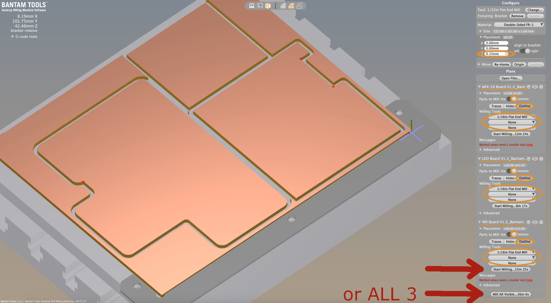
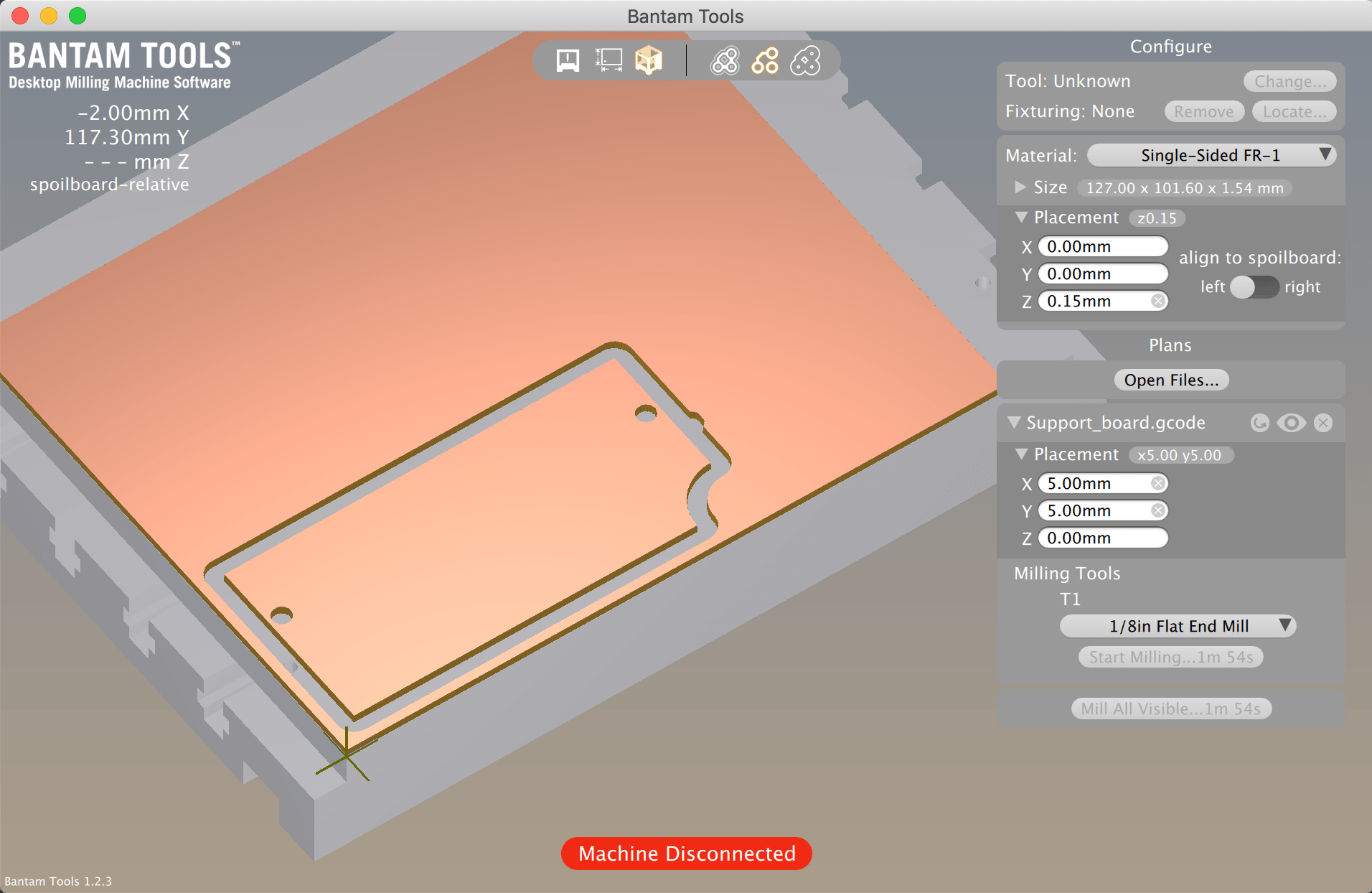
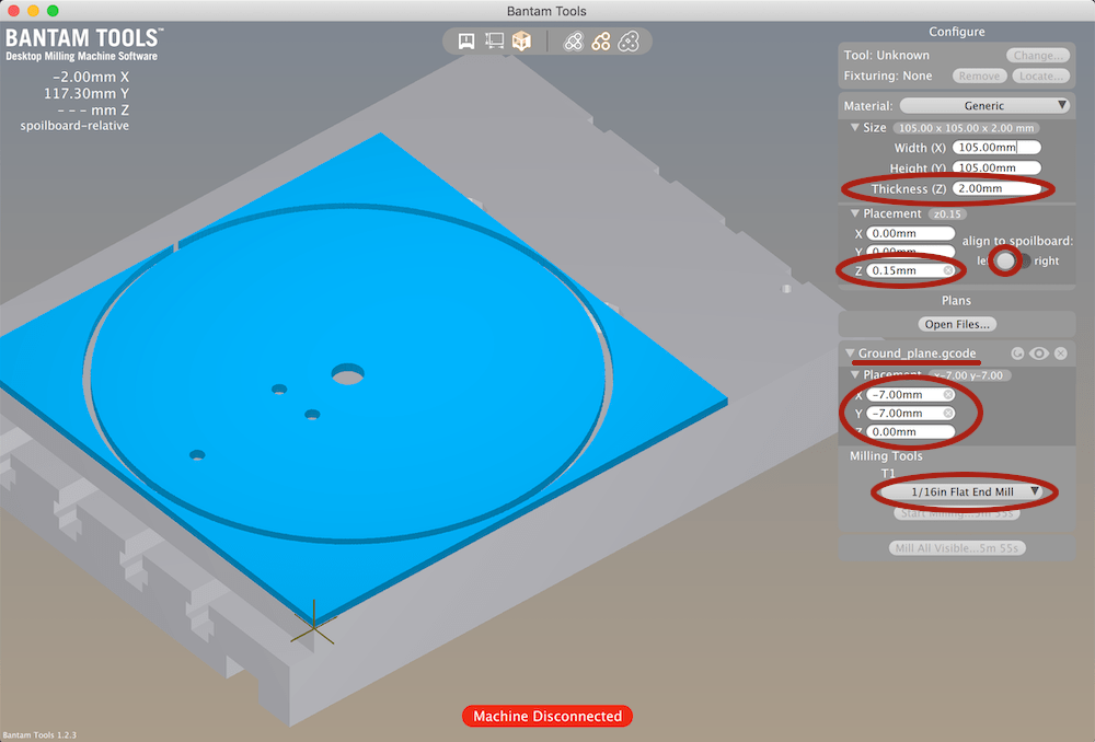
13.12. Access the Velodyne VLP-16
Warning
The reader’s computer needs to be physically connected to the OpenMMS sensor using an ethernet cable and assigned an appropriate static IP address and subnet mask to connect successfully to the VLP-16. An IP address of 192.168.1.23 and a subnet mask of 255.255.255.0 are recommended.
As discussed in section 8.7, the Velodyne VLP-16 lidar sensor provides the user with a Web-based User Interface (WebUI) to access the sensor’s settings. Unlike the APX-18, the VLP-16 does not store its observations internally. Rather, the VLP-16 streams its observations over TCP/UDP, which the Raspberry Pi computer is programmed to collect and store. Therefore, there is no requirement to access the VLP-16’s WebUI after each data collection campaign. However, now that the OpenMMS sensor has been fully assembled, it is good to check that the VLP-16 correctly receives the Pulse-Per-Second (PPS) signal and the corresponding NMEA RMC message from the APX-18. Without this information, the VLP-16 lidar observations will not be able to be fused with the position and orientation observations from the APX-18.
The OpenMMS sensor needs to be powered on, and the APX-18 needs to be receiving adequate GNSS signals (i.e., has a clear view of the sky) before the VLP-16 will collect the required UTC supplementary data. The VLP-16 is powered on by merely starting a typical data collection campaign. To connect to the VLP-16’s WebUI, open a web browser on the connected computer and enter the address of 192.168.1.201 into the URL textbox and press enter. No login information is required. At the very bottom of the WebUI’s main page, there is a GPS Position textbox and a PPS textbox. If the VLP-16 is receiving the PPS signal from the APX-18, the PPS textbox will display Locked. If it is receiving the NMEA RMC message from the APX-18, the GPS Position textbox will display the user’s current position (latitude and longitude), see the figure below.
Tip
If the PPS textbox displays Locked but the GPS Position textbox remains empty, the first thing to check is that the Report legacy talker id checkbox is checked for the Serial1/COM1 port on the APX-18 (refer to Figure 8.6-14 for details).
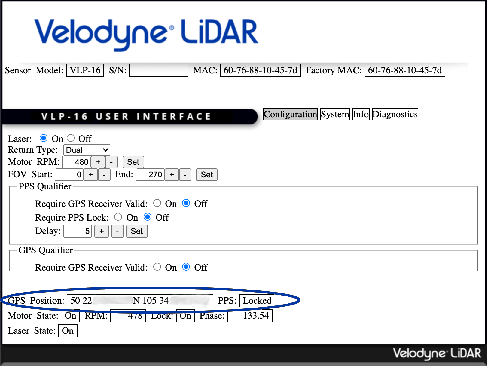
Fig 13.12-1. VLP-16’s WebUI showing good PPS and NMEA RMC data
Important
Refer to the complete set of documentation provided by Velodyne or contact their Technical Support team for further details.
13.13. Access the Livox MID-40
Warning
The reader’s computer needs to be physically connected to the OpenMMS sensor using an ethernet cable and assigned an appropriate static IP address and subnet mask to connect successfully to the MID-40. An IP address of 192.168.1.23 and a subnet mask of 255.255.255.0 are recommended.
As discussed in section 8.8, the Livox MID-40 lidar sensor does NOT provide the user with a Web-based User Interface (WebUI) to access the sensor’s settings. Unlike the APX-18, the MID-40 does not store its observations internally. Rather, the MID-40 streams its observations over TCP/UDP, which the Raspberry Pi computer is programmed to collect and store. Therefore, there is no requirement to directly access the MID-40 after each data collection campaign. However, now that the OpenMMS sensor has been fully assembled, it is good to check that the MID-40 correctly receives the Pulse-Per-Second (PPS) signal from the APX-18. Without this information the MID-40 lidar observations will not be able to be fused with the position and orientation observations from the APX-18.
The OpenMMS sensor needs to be powered on, and the APX-18 needs to be receiving adequate GNSS signals (i.e., has a clear view of the sky) before the MID-40 will receive the required UTC supplementary data. Next, open the Livox Viewer application and ensure the correct network adapter is selected within the Network Adapter menu at the top of the screen. Next, powered on the MID-40 by starting a typical data collection campaign. From the moment the Lidar LED turns on, there is a 20 second window of time where the MID-40 will be available within the Livox Viewer application. Find the sensor within the left column and then slide the radio button to the right to connect to the MID-40 sensor. After the 20 second window of time has elapsed the MID-40 will connect to the Raspberry Pi computer inside the OpenMMS sensor and will no longer be available within the Livox Viewer application. Lastly, click on the ‘Gear’ icon inside of Livox Viewer and within the Settings dialog window that appears, examine the PPS State parameter. If a valid PPS signal is being received the parameter will report, PPS Signal. If no PPS signal is received the parameter will report, NO PPS (see the figure below).
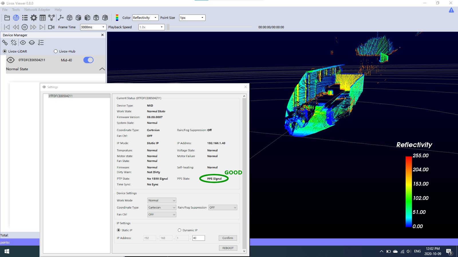
Fig 13.13-1. MID-40 reporting good PPS signal
13.14. Data Collection Checklist
The following checklist describes the recommended procedure to follow when collecting digital mapping data using the OpenMMS sensor V1.3. Click Here to download a PDF version of the checklist.

Fig 13.14-1. Recommended Data Collection Checklist
Upon completing a typical OpenMMS data collection campaign, the following digital mapping datasets should have been downloaded from the sensor and stored on the user’s computer.
Precise position, orientation, and camera event data - Applanix proprietary .T04 binary file downloaded from the APX-18 sensor.
Approximate position, orientation, and camera event data - .TRAJ ascii file downloaded from RPi computer.
Lidar observations - .PCAP binary file downloaded from the RPi computer.
Nadir view photos - typically several hundred .JPG binary files downloaded from the Sony A6000 camera’s SD card.
Nadir view video (optional) - .MP4 binary file downloaded from the RPi computer.
Time sync information - .LIVOX ascii file downloaded from RPi computer (only for systems with a Livox MID-40 sensor)

Fig 13.14-2. Typical OpenMMS collected datasets